From Dataset to Biological Signature

1 Biological signature

A biological signature is a fixed gene list with weights and a decision threshold, fit to answer a specific classification question. Every reported performance number is conditional on the data having selected those genes.

This post runs Golub et al. (1999) ALL/AML microarray data end to end: recover the original train/test split, fit an elastic-net signature without leakage, and report honest external validation. The pipeline is described twice — ML vocabulary and statistical vocabulary.

Primer without code: What is a Biological Signature?.

2 Biology background

Acute lymphoblastic leukemia (ALL) and acute myeloid leukemia (AML) require opposite treatments. Pre-1999 diagnosis used morphology, cytochemistry, and surface markers.

Bone marrow stem cell gives two lines:

flowchart TD
  S["Bone marrow stem cell"] --> L["Lymphoid line<br/>B-cells, T-cells"]
  S --> M["Myeloid line<br/>red cells, platelets, granulocytes"]
  L -->|glitch| ALL["<b>ALL</b><br/>lymphoblasts"]
  M -->|glitch| AML["<b>AML</b><br/>myeloblasts"]

• ALL: lymphoid line jammed; commonest childhood cancer.
• AML: myeloid line jammed; adult disease; affects oxygen transport and clotting faster.

Diagnostic question: which line is stuck?

3 Data provenance

Source: Golub et al. (1999), Whitehead Institute / Dana-Farber. 72 acute leukemia patients; Affymetrix HU6800 array (7,129 gene probes). Archived hospital samples; goal was to show tumour type is legible in gene expression.

• Matrix used here: Efron and Hastie’s CASI data page (leukemia_big.csv.gz), cached in data/.
• Split key: original Whitehead files (golub_train.csv.gz, golub_independent.csv.gz) carry probe accessions and patient IDs the CASI copy dropped.
• Objective: classify ALL vs AML from expression.
• Downstream impact: treatment assignment (vincristine/steroids vs cytarabine/anthracycline). Target metric: performance at a different hospital, not peak training accuracy.

import warnings
import numpy as np
import pandas as pd
import matplotlib.pyplot as plt
from scipy.stats import beta

warnings.filterwarnings("ignore")
rng_seed = 0

plt.rcParams.update({
    "figure.dpi": 150, "savefig.bbox": "tight", "font.size": 9,
    "axes.spines.top": False, "axes.spines.right": False,
    "axes.grid": True, "grid.alpha": 0.25, "axes.axisbelow": True,
})
ALL_C, AML_C = "#1D5C6E", "#C98A12"

# The CASI matrix: 7,128 genes x 72 samples, column names carry the labels.
casi = pd.read_csv("data/leukemia_big.csv.gz")
X = casi.to_numpy().T                                    # samples x genes
y = np.array([int(c.split(".")[0].startswith("AML")) for c in casi.columns])

# The original Whitehead files, used only as a key: they carry the Affymetrix
# probe accessions and the per-patient sample IDs that the CASI copy dropped.
def read_golub(path):
    d = pd.read_csv(path)
    ids = [c for c in d.columns[2:] if not c.startswith("call")]
    return d["Gene Accession Number"].to_numpy(), d["Gene Description"].to_numpy(), \
           d[ids].to_numpy(dtype=float), ids

acc, desc, G_train, id_train = read_golub("data/golub_train.csv.gz")
_, _, G_test, id_test = read_golub("data/golub_independent.csv.gz")
truth = pd.read_csv("data/golub_labels.csv").set_index("patient")["cancer"].to_dict()

print(f"expression matrix : {X.shape[0]} samples x {X.shape[1]} genes")
print(f"class balance     : {(y==0).sum()} ALL, {y.sum()} AML")

expression matrix : 72 samples x 7128 genes
class balance     : 47 ALL, 25 AML

72 samples × 7,128 genes (\(p \gg n\)).

pd.DataFrame(
    X[:5, :6].round(3),
    index=[f"sample {i} ({'AML' if y[i] else 'ALL'})" for i in range(5)],
    columns=[f"gene {j}" for j in range(6)],
)

	gene 0	gene 1	gene 2	gene 3	gene 4	gene 5
sample 0 (ALL)	-1.534	-1.236	-0.334	0.489	-1.301	-1.683
sample 1 (ALL)	-0.868	-1.276	0.376	0.444	-1.230	-1.642
sample 2 (ALL)	-0.433	-1.184	-0.459	0.436	-1.326	-1.407
sample 3 (ALL)	-1.672	-1.596	-1.423	0.193	-1.818	-1.744
sample 4 (ALL)	-1.188	-1.335	-0.797	0.236	-1.311	-1.654

Each patient column is z-scored (mean 0, SD 1). Per-gene preprocessing across patients is undocumented (“lost in time”).

4 Train/test split recovery

Golub’s design:

• 38 training: single hospital, bone marrow, predictor built here.
• 34 external test: later collection, different labs, some blood — simulates new hospital.

CASI file lacks patient IDs. Recovery method: column-wise rank order is invariant to affine rescaling → Spearman rank correlation matches CASI columns to Golub patients.

G = np.hstack([G_train, G_test])[:X.shape[1]]   # CASI drops Golub's last probe
ids = id_train + id_test
golub_y = np.array([int(truth[int(i)] == "AML") for i in ids])

rank = lambda A: np.argsort(np.argsort(A, axis=0), axis=0).astype(float)
Rc, Rg = rank(casi.to_numpy()), rank(G)
Rc = (Rc - Rc.mean(0)) / Rc.std(0)
Rg = (Rg - Rg.mean(0)) / Rg.std(0)
S = (Rc.T @ Rg) / G.shape[0]                    # 72 x 72 Spearman matrix
match, best = S.argmax(1), np.sort(S, axis=1)

print(f"unique matches      : {len(set(match.tolist()))}/72")
print(f"labels agree        : {(golub_y[match] == y).sum()}/72")
print(f"worst true match    : {best[:, -1].min():.3f}")
print(f"best runner-up      : {best[:, -2].max():.3f}")
print(f"CASI column 0 -> patient {ids[match[0]]};  column 34 -> patient {ids[match[34]]}")

unique matches      : 72/72
labels agree        : 72/72
worst true match    : 0.945
best runner-up      : 0.884
CASI column 0 -> patient 39;  column 34 -> patient 1

• 72/72 unique matches; all labels agree.
• Worst true match: 0.945; best wrong candidate: 0.884.
• CASI stores 34 external samples first (columns 0–33), training second (34–71).

4.1 Preprocessing caveat

Undocumented per-gene step may have pooled all 72 patients. Column z-scoring is safe; pooled gene normalization would leak test into training. All results below are conditional on column scaling only.

test_ix, train_ix = np.arange(34), np.arange(34, 72)
probe = {a: i for i, a in enumerate(acc[:X.shape[1]])}
mpo, ccnd3 = probe["M19507_at"], probe["M92287_at"]

Z = (X - X.mean(0)) / (X.std(0) + 1e-9)
U, sv, _ = np.linalg.svd(Z - Z.mean(0), full_matrices=False)
pcs = U[:, :5] * sv[:5]

# Pick the axes by what they actually carry, rather than assuming PC1/PC2:
# correlate each component with class and with cohort membership.
cohort = np.r_[np.zeros(34), np.ones(38)]
corr = lambda v: np.array([abs(np.corrcoef(v, pcs[:, k])[0, 1]) for k in range(5)])
k_cls, k_coh = corr(y).argmax(), corr(cohort).argmax()

fig, (a1, a2) = plt.subplots(1, 2, figsize=(8, 3.6))
for cls, name, col in [(0, "ALL", ALL_C), (1, "AML", AML_C)]:
    m = y == cls
    a1.scatter(X[m, ccnd3], X[m, mpo], c=col, s=28, alpha=0.85, label=name,
               edgecolor="white", linewidth=0.5)
a1.set(xlabel="CCND3 (cyclin D3), lymphoid", ylabel="MPO (myeloperoxidase), myeloid",
       title="Two genes")
a1.legend(frameon=False, fontsize=8)

for cls, col in [(0, ALL_C), (1, AML_C)]:
    for ix, mark, lab in [(train_ix, "o", "training"), (test_ix, "^", "external")]:
        m = np.intersect1d(np.flatnonzero(y == cls), ix)
        a2.scatter(pcs[m, k_cls], pcs[m, k_coh], c=col, marker=mark, s=28, alpha=0.85,
                   edgecolor="white", linewidth=0.5,
                   label=f"{'AML' if cls else 'ALL'}, {lab}")
a2.set(xlabel=f"PC{k_cls + 1}  (carries class, |r| = {corr(y)[k_cls]:.2f})",
       ylabel=f"PC{k_coh + 1}  (carries cohort, |r| = {corr(cohort)[k_coh]:.2f})",
       title="Colour = class, shape = cohort")
a2.legend(frameon=False, fontsize=7, loc="best")
fig.tight_layout()
plt.show()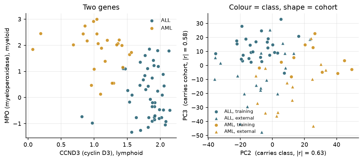

Figure 1: Left: two genes named later in the post, one myeloid and one lymphoid, separate the classes almost on their own. Right: the component that carries diagnosis plotted against the one that carries cohort. Class separates left-to-right and the laboratory separates bottom-to-top, on different axes — the nuisance variable has structure of its own.

• CCND3 (lymphoid) vs MPO (myeloid) nearly separate classes alone.
• Class and cohort load on different principal components. Ridge classifier on cohort alone: 78% CV accuracy.

5 ML pipeline

5.1 Input representation

Model sees samples × genes matrix. Biology (probe mapping, normalization) is upstream and assay-specific.

5.2 Supervised signature

Signature requires labels (ALL vs AML). Unsupervised structure ≠ signature without a question. Golub (1999) also did class discovery then prediction; discovery proposes the question, prediction remains supervised.

5.3 Elastic net objective

Shipped artifact: fixed gene list, weights, threshold — locked before opening test set.

\[ \hat\beta \;=\; \arg\min_{\beta}\; -\frac{1}{n}\sum_{i=1}^{n}\Big[y_i\,x_i^{\top}\beta - \log\big(1 + e^{x_i^{\top}\beta}\big)\Big] \;+\; \lambda\Big(\alpha\lVert\beta\rVert_1 + \tfrac{1-\alpha}{2}\lVert\beta\rVert_2^2\Big) \]

• L1 (\(\lVert\beta\rVert_1\)): sparsity; exact zeros.
• L2 (\(\lVert\beta\rVert_2^2\)): groups correlated genes.
• \(\alpha = 0.5\); tune \(\lambda\) (via \(C = 1/\lambda\)) by nested cross-validation on 38 training samples only.

from sklearn.linear_model import LogisticRegression
from sklearn.model_selection import StratifiedKFold, cross_val_score
from sklearn.metrics import accuracy_score, roc_auc_score, brier_score_loss

Xtr, ytr, Xte, yte = X[train_ix], y[train_ix], X[test_ix], y[test_ix]
Cs = np.logspace(-2, 1, 7)

def enet(C):
    return LogisticRegression(penalty="elasticnet", solver="saga", l1_ratio=0.5,
                              C=C, max_iter=3000, tol=1e-3, random_state=rng_seed)

def screen(A, k=2000):
    """Unsupervised variance screen. Never sees y, so it is safe inside a fold."""
    return np.argsort(-A.var(0))[:k]

outer, scores = StratifiedKFold(5, shuffle=True, random_state=0), []
for a, b in outer.split(Xtr, ytr):
    g = screen(Xtr[a])
    mu, sd = Xtr[a][:, g].mean(0), Xtr[a][:, g].std(0) + 1e-9
    Za, Zb = (Xtr[a][:, g] - mu) / sd, (Xtr[b][:, g] - mu) / sd
    inner = StratifiedKFold(4, shuffle=True, random_state=1)
    C = max(Cs, key=lambda c: cross_val_score(enet(c), Za, ytr[a], cv=inner).mean())
    scores.append(accuracy_score(ytr[b], enet(C).fit(Za, ytr[a]).predict(Zb)))

# Full-training-set path, for the figure and for the final penalty.
g = screen(Xtr)
mu, sd = Xtr[:, g].mean(0), Xtr[:, g].std(0) + 1e-9
Ztr, Zte = (Xtr[:, g] - mu) / sd, (Xte[:, g] - mu) / sd
cv5 = StratifiedKFold(5, shuffle=True, random_state=1)
path = np.array([cross_val_score(enet(c), Ztr, ytr, cv=cv5) for c in Cs])
C_star = Cs[path.mean(1).argmax()]

print(f"nested CV accuracy : {np.mean(scores):.3f}  (outer folds "
      f"{[round(s, 2) for s in scores]})")

fig, ax = plt.subplots(figsize=(6.2, 3.2))
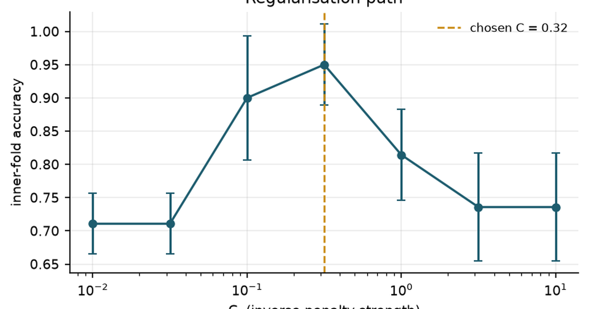
ax.errorbar(Cs, path.mean(1), yerr=path.std(1), marker="o", color=ALL_C,
            capsize=3, linewidth=1.5, markersize=5)
ax.axvline(C_star, color=AML_C, linestyle="--", linewidth=1.3,
           label=f"chosen C = {C_star:.2f}")
ax.set(xscale="log", xlabel="C  (inverse penalty strength)",
       ylabel="inner-fold accuracy", title="Regularisation path")
ax.legend(frameon=False, fontsize=8)
plt.show()

nested CV accuracy : 0.921  (outer folds [0.75, 1.0, 1.0, 0.86, 1.0])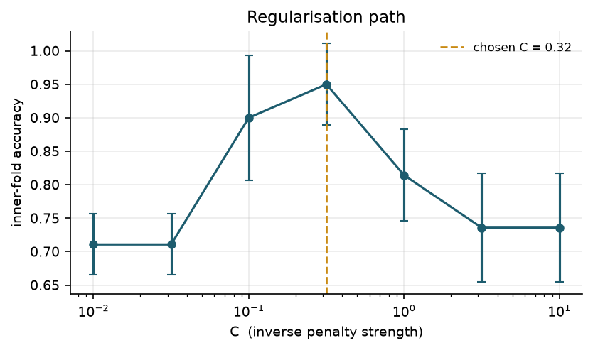

Figure 2: Inner-fold accuracy along the regularisation path, on the 38 training samples only. Accuracy peaks at a single interior value. To the left the penalty is strong enough to zero out genes the model needs; to the right it is weak enough to admit genes that only help on the training fold. Error bars are one standard deviation across five folds, and they are wide — 38 samples do not locate this optimum precisely.

Nested CV training accuracy: 0.921. External test (once):

final = enet(C_star).fit(Ztr, ytr)
selected = g[np.flatnonzero(final.coef_[0])]
p_test = final.predict_proba(Zte)[:, 1]

print(f"genes with non-zero coefficient : {len(selected)}")
print(f"external accuracy : {accuracy_score(yte, p_test > 0.5):.3f} "
      f"({int((( p_test > 0.5) == yte).sum())}/34)")
print(f"external AUC      : {roc_auc_score(yte, p_test):.3f}")
print(f"external Brier    : {brier_score_loss(yte, p_test):.3f}")
wrong = np.flatnonzero((p_test > 0.5).astype(int) != yte)
print(f"the one error     : predicted p(AML) = {p_test[wrong][0]:.3f}")

genes with non-zero coefficient : 88
external accuracy : 0.971 (33/34)
external AUC      : 1.000
external Brier    : 0.041
the one error     : predicted p(AML) = 0.468

Results:

• 33/34 correct; AUC 1.000 (perfect ranking); one error at \(p = 0.468\).
• Training CV (0.921) understated external performance (0.971).

lineage = {
    "M19507_at": "MPO, myeloperoxidase — the granulocyte enzyme",
    "M23197_at": "CD33 — myeloid surface antigen",
    "X52056_at": "SPI1 / PU.1 — myeloid master transcription factor",
    "M84526_at": "DF, adipsin — Golub's AML-high list",
    "M27891_at": "CST3, cystatin C — Golub's AML-high list",
    "M92287_at": "CCND3, cyclin D3 — Golub's ALL-high list",
    "U05259_rna1_at": "MB-1 / CD79a — B-cell receptor component",
    "M31523_at": "TCF3 / E2A — required for B-cell development",
}
hits = [(acc[i], lineage[acc[i]]) for i in selected if acc[i] in lineage]
for a, note in hits:
    print(f"  {a:16s} {note}")
print(f"\n{len(hits)} of these annotated markers survived selection.")

  M27891_at        CST3, cystatin C — Golub's AML-high list
  X52056_at        SPI1 / PU.1 — myeloid master transcription factor
  M84526_at        DF, adipsin — Golub's AML-high list
  M19507_at        MPO, myeloperoxidase — the granulocyte enzyme
  U05259_rna1_at   MB-1 / CD79a — B-cell receptor component
  M23197_at        CD33 — myeloid surface antigen
  M92287_at        CCND3, cyclin D3 — Golub's ALL-high list

7 of these annotated markers survived selection.

Selected genes: myeloid vs lymphoid markers; includes MPO (pre-1999 stain target).

6 Statistical pipeline

Same procedure; emphasis on inference under \(p \gg n\) and post-selection bias.

6.1 Post-selection inference

Selected gene weights inherit selection luck. Standard CIs assume pre-specified variables. Repairs:

1. Split sample: select on one half, infer on other.
2. Selective inference: correct for selection.
3. Knockoffs: fake genes through same contest.

6.2 False discovery rate

7,128 tests at 5% → ~356 false positives by chance. FDR controls expected fraction wrong among reported genes:

\[ \mathrm{FDR} \;=\; \mathbb{E}\!\left[\frac{V}{\max(R, 1)}\right] \]

Benjamini–Hochberg delivers long-run FDR control when genes correlate; single-list fraction can swing (gene gangs).

6.3 Pipeline stages

1. Pre-specify estimand and threshold.
2. Split before any transformation.
3. Fit scaling and gene filter on training folds only.
4. Inner loop: choose penalty; outer loop: score performance.
5. Stability selection across subsamples.
6. Lock model; test externally once; report intervals and calibration.

Step 3 is most commonly violated.

6.4 Leakage demonstration

Score all genes on full data, keep top 50, then cross-validate → held-out fold influenced gene choice. Ambroise and McLachlan (2002).

def top_genes(A, lab, k=50):
    m0, m1 = A[lab == 0].mean(0), A[lab == 1].mean(0)
    se = np.sqrt(A[lab == 0].var(0) / (lab == 0).sum()
                 + A[lab == 1].var(0) / lab.sum()) + 1e-9
    return np.argsort(-np.abs((m1 - m0) / se))[:k]

def two_ways(lab, cv=StratifiedKFold(10, shuffle=True, random_state=7)):
    once = cross_val_score(enet(1.0), Z[:, top_genes(Z, lab)], lab, cv=cv).mean()
    fold = [accuracy_score(lab[b], enet(1.0)
            .fit(Z[a][:, (gi := top_genes(Z[a], lab[a]))], lab[a])
            .predict(Z[b][:, gi])) for a, b in cv.split(Z, lab)]
    return 1 - once, 1 - np.mean(fold)

opt, honest = two_ways(y)
print(f"real labels     : filter once {opt:.1%} error | filter in fold {honest:.1%}")

shuffled = np.random.default_rng(3).permutation(y)
opt_n, honest_n = two_ways(shuffled)
print(f"labels shuffled : filter once {opt_n:.1%} error | filter in fold {honest_n:.1%}")
print(f"chance for this class balance : {(y == 0).mean():.1%} correct by always saying ALL")

real labels     : filter once 2.9% error | filter in fold 4.3%
labels shuffled : filter once 7.0% error | filter in fold 33.2%
chance for this class balance : 65.3% correct by always saying ALL

Real labels: 2.9% (leaked) vs 4.3% (honest) — small gap because signal is strong.

Shuffled labels: 7.0% error (93% accuracy on noise) vs 33.2% (honest) ≈ always-ALL baseline.

6.5 Stability selection

100 half-samples of 38 training patients; fixed penalty; count reselection frequency.

rng = np.random.default_rng(rng_seed)
freq, B = np.zeros(X.shape[1]), 100
pool = screen(Xtr)
for _ in range(B):
    take = rng.choice(len(ytr), len(ytr) // 2, replace=False)
    if len(np.unique(ytr[take])) < 2:
        continue
    A = Xtr[take][:, pool]
    A = (A - A.mean(0)) / (A.std(0) + 1e-9)
    freq[pool[np.flatnonzero(enet(0.5).fit(A, ytr[take]).coef_[0])]] += 1
freq /= B

order = np.argsort(-freq)
for t in (0.5, 0.6, 0.7, 0.9):
    print(f"selection frequency >= {t}: {(freq >= t).sum()} genes")

fig, ax = plt.subplots(figsize=(7.6, 3.4))
top = order[:60]
ax.bar(range(len(top)), freq[top], color=ALL_C, width=0.8)
ax.axhline(0.6, color=AML_C, linestyle="--", linewidth=1.3, label="cutoff = 0.6")
above = int((freq[top] >= 0.6).sum())
ax.set_xticks(range(above))
ax.set_xticklabels([acc[i] for i in top[:above]], rotation=90, fontsize=5)
ax.set(xlim=(-1, len(top)), ylabel="selection frequency",
       xlabel="genes, ranked", title=f"{B} half-samples of the 38 training patients")
ax.legend(frameon=False, fontsize=8)
plt.show()

selection frequency >= 0.5: 45 genes
selection frequency >= 0.6: 33 genes
selection frequency >= 0.7: 26 genes
selection frequency >= 0.9: 12 genes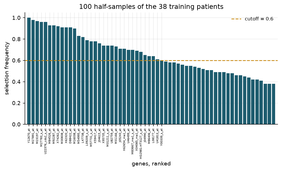

Figure 3: Selection frequency across 100 half-samples of the training cohort, sorted. The dashed line is a 0.6 cutoff. Genes above it are labelled by Affymetrix probe.

45 genes ≥50% frequency; 12 ≥90%. Gene list is one draw, not a fixed biological object.

6.6 Golub-50 comparison

Reconstruct Golub’s 50-gene predictor (\(P(g,c) = (\mu_1 - \mu_0)/(\sigma_1 + \sigma_0)\)); compare raw vs log10-clipped preprocessing.

def snr(A, lab):
    d = A[lab == 1].mean(0) - A[lab == 0].mean(0)
    return d / (A[lab == 1].std(0, ddof=1) + A[lab == 0].std(0, ddof=1) + 1e-12)

raw = G_train.T
P_raw = snr(raw, golub_y[:38])
P_log = snr(np.log10(np.clip(raw, 100, 16000)), golub_y[:38])
fifty = lambda P: set(np.argsort(-P)[:25]) | set(np.argsort(P)[:25])
g50_raw, g50_log = fifty(P_raw), fifty(P_log)

print(f"Golub-50, raw vs his own log10 preprocessing : {len(g50_raw & g50_log)}/50 shared")
print(f"elastic net set vs Golub-50 (log10)         : "
      f"{len(set(selected) & g50_log)} of 50 genes in common")
print("top AML-high probes:",
      ", ".join(acc[i] for i in np.argsort(-P_log)[:4]))

Golub-50, raw vs his own log10 preprocessing : 32/50 shared
elastic net set vs Golub-50 (log10)         : 26 of 50 genes in common
top AML-high probes: M27891_at, X95735_at, U50136_rna1_at, M23197_at

Log preprocessing alone changes 18/50 genes. Elastic net agrees with Golub-50 on 26/50.

7 External validation limits

33/34 external accuracy is real but \(n = 34\).

def wilson(k, n, z=1.96):
    c = (k / n + z * z / (2 * n)) / (1 + z * z / n)
    h = z * np.sqrt(k / n * (1 - k / n) / n + z * z / (4 * n * n)) / (1 + z * z / n)
    return c - h, c + h

print(f"external accuracy 33/34   : 95% CI [{wilson(33, 34)[0]:.3f}, {wilson(33, 34)[1]:.3f}]")
print(f"nested CV, 35/38          : 95% CI [{wilson(35, 38)[0]:.3f}, {wilson(35, 38)[1]:.3f}]")

sens, fpr_hi = 13 / 14, beta.ppf(0.975, 1, 20)
print(f"\nspecificity 20/20, but 95% upper bound on the false-positive rate: {fpr_hi:.3f}")
for prev, where in [(0.35, "suspected leukemia at referral"), (0.02, "a broader haematology clinic")]:
    ppv = sens * prev / (sens * prev + fpr_hi * (1 - prev))
    print(f"  prevalence {prev:>5.0%} ({where}): PPV could be as low as {ppv:.2f}")

external accuracy 33/34   : 95% CI [0.851, 0.995]
nested CV, 35/38          : 95% CI [0.792, 0.973]

specificity 20/20, but 95% upper bound on the false-positive rate: 0.168
  prevalence   35% (suspected leukemia at referral): PPV could be as low as 0.75
  prevalence    2% (a broader haematology clinic): PPV could be as low as 0.10

• 33/34 → 95% CI [0.851, 0.995] for true accuracy.
• 0/20 false AML calls → consistent with FPR up to ~17%.
• PPV at 35% prevalence (referral): could be as low as ~0.75.
• PPV at 2% prevalence (general clinic): could be as low as ~0.10.

Accuracy is a property of model and population. Signature answers “ALL or AML among patients known to have one of them.”

8 References

Biology and genomics

• Golub, T. R. et al. (1999). Molecular classification of cancer: class discovery and class prediction by gene expression monitoring. Science 286:531–537.
• Alizadeh, A. A. et al. (2000). Distinct types of diffuse large B-cell lymphoma identified by gene expression profiling. Nature 403:503–511.
• van ’t Veer, L. J. et al. (2002). Gene expression profiling predicts clinical outcome of breast cancer. Nature 415:530–536.
• Subramanian, A. et al. (2005). Gene set enrichment analysis: a knowledge-based approach for interpreting genome-wide expression profiles. PNAS 102:15545–15550.
• Leek, J. T. et al. (2010). Tackling the widespread and critical impact of batch effects in high-throughput data. Nature Reviews Genetics 11:733–739.
• Whalen, S. et al. (2022). Navigating the pitfalls of applying machine learning in genomics. Nature Reviews Genetics 23:169–181.

Statistics and machine learning

• Tibshirani, R. (1996). Regression shrinkage and selection via the lasso. JRSS-B 58:267–288.
• Benjamini, Y. & Hochberg, Y. (1995). Controlling the false discovery rate: a practical and powerful approach to multiple testing. JRSS-B 57:289–300.
• Zou, H. & Hastie, T. (2005). Regularization and variable selection via the elastic net. JRSS-B 67:301–320.
• Guyon, I., Weston, J., Barnhill, S. & Vapnik, V. (2002). Gene selection for cancer classification using support vector machines. Machine Learning 46:389–422.
• Dudoit, S., Fridlyand, J. & Speed, T. P. (2002). Comparison of discrimination methods for the classification of tumors using gene expression data. JASA 97:77–87.
• Ambroise, C. & McLachlan, G. J. (2002). Selection bias in gene extraction on the basis of microarray gene-expression data. PNAS 99:6562–6566.
• Meinshausen, N. & Bühlmann, P. (2010). Stability selection. JRSS-B 72:417–473.
• Barber, R. F. & Candès, E. J. (2015). Controlling the false discovery rate via knockoffs. Annals of Statistics 43:2055–2085.
• Candès, E., Fan, Y., Janson, L. & Lv, J. (2018). Panning for gold: ‘model-X’ knockoffs for high-dimensional controlled variable selection. JRSS-B 80:551–577.
• Efron, B. & Hastie, T. (2016). Computer Age Statistical Inference: Algorithms, Evidence, and Data Science. Cambridge University Press.

Data. The expression matrix is leukemia_big.csv from the CASI data page. Probe accessions and sample identifiers come from the original Whitehead files, data_set_ALL_AML_train.csv and data_set_ALL_AML_independent.csv; the URL cited in the 1999 paper is long dead, so this post uses a mirror of them. Both are cached under data/ by src/fetch_data.py.