Explainability is Not Causality: What is not Why

Attribution names what a fitted model did on one input. A causal claim names what would happen in the world if you changed something.

Attribution methods assign credit for one prediction across input features. A long SHAP bar for tenure is a fact about a fitted model. It does not imply that extending tenure would change churn.

The two fields share vocabulary (why, because, important, counterfactual) and answer different questions.

1 Demonstration: husky versus wolf

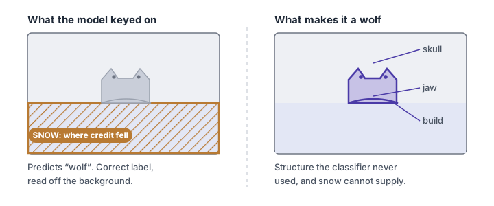
Ribeiro, Singh & Guestrin (2016) trained a husky-versus-wolf classifier on 20 images chosen so every wolf had snow in the background and no husky did.

Husky (left), wolf (right) — the two categories a classifier is about to be asked to tell apart.

Asked which pixels it used, the model named snow. That attribution is accurate as a description of the fitted association. Snow does not make an animal a wolf.

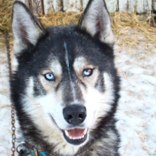
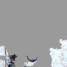
(a) A husky the classifier called a wolf.

(b) The evidence it kept: mostly snow, with the collar and a scrap of muzzle surviving.

Reproduced from Ribeiro, Singh & Guestrin (2016), Figure 11, for commentary. Shown only predictions, 10 of 27 graduate students trusted this classifier; shown the explanation, 3 did, and those naming snow as its evidence rose from 12 to 25.

On an uncurated training set that pattern can appear (background, watermark, collection artifact). The attribution chart looks the same whether the named feature is the mechanism or the accident.

What the explanation cannot reach: the structure that makes the animal a wolf.

2 Explainability

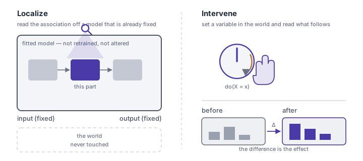
Attribution answers: given this model and this input, which parts account for the output?

Methods differ in what counts as a part:

Saliency: pixels scored by how much a nudge would move the output.
SHAP / LIME: credit among features. LIME fits a simple local stand-in and reads the explanation off that stand-in.
Attention visualisation: tokens the model weighted.

Scope:

one fitted model (held fixed)
one instance
one prediction

The procedure does not consult the world. It cannot distinguish a real mechanism from a collection artifact.

Localizing points a spotlight inside a model that stays fixed. Intervening changes the world and reads the difference.

3 Causality

A causal claim is obtained by intervening: set a variable rather than observe it, then measure what moves.

Instruments:

randomized trial
A/B test
natural experiment when neither can be run

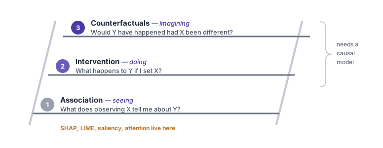
Pearl’s ladder (three non-substitutable question types):

Seeing — what co-occurs with what.
Doing — what follows if a variable is set.
Imagining otherwise — what would have happened to this unit had things differed.

No amount of seeing-data answers a doing-question without assumptions brought in from outside the data.

Cost asymmetry: localization is one forward pass on a model already on disk. Intervention requires changing the world.

Pearl’s ladder of causation. Attribution lives on rung one; every rung above needs a causal model.

4 Shared vocabulary

Field	Method	Question it answers	What it does
Explainability (“what”)	Feature attribution (SHAP, LIME, Integrated Gradients)	“What inputs drove this prediction?”	Assigns credit/weight to each input feature for a specific output
	Saliency maps / Grad-CAM	“What part of the input did the model look at?”	Highlights regions (e.g. pixels) with highest influence on output
	Attention visualization	“What did the model attend to?”	Surfaces attention weights in transformer-style models
	Surrogate models	“What simple rule approximates this decision?”	Builds an interpretable stand-in for a local region of behavior
	Counterfactual explanations (ML sense)	“What’s the smallest input change that flips the output?”	Finds a minimally-different input the model classifies differently
	Concept activation vectors (TCAV)	“What human-understandable concept does this correspond to?”	Tests whether a learned direction in activation space aligns with a concept
Causality (“why”)	Randomized controlled trials (RCTs)	“Does X cause Y?”	Physically intervenes on X (randomly) to rule out confounding
	Causal graphs / DAGs (Pearl)	“What’s the causal structure connecting these variables?”	Encodes assumed cause-effect relationships
	Do-calculus (Pearl)	“What happens if we intervene on X?”	Formal rules for computing intervention effects from observational data + a causal graph
	Instrumental variables	“Does X cause Y, despite unmeasured confounding?”	Uses a variable affecting X but not Y directly, to isolate the causal effect
	Difference-in-differences / Regression discontinuity	“Did this policy/event cause the change?”	Exploits natural experiments to approximate randomization
	Counterfactual reasoning (Pearl’s rung 3)	“Would Y have happened if X hadn’t?”	Uses a fitted causal model to answer individual-level counterfactuals

The two counterfactual rows share a name and sit on different rungs:

ML counterfactual: nearest input the model labels differently. Fact about a decision boundary (rung 1).
Pearl counterfactual: what would have happened to this unit under a different treatment. Requires a structural model (rung 3).

5 Causal claims about a network

A causal claim about the network (not about the world) is obtained by intervening on internals:

delete a concept from the representation and re-run the forward pass
paste activations from one input into another input’s forward pass (activation patching) and measure output change

That is distinct from an ML counterfactual, which searches inputs. Whether the world works the same way is a separate question.

6 Scope

Explainability: what a fitted model did, for one input.
Causality: what happens in the world under intervention.

Reading the first as the second is a category error. Tenure’s long bar does not license a tenure-extension policy; that requires intervening on tenure.

Attribution. Describes. Models. Intervention. Describes. Worlds. Confusing. Them. Licenses. Bad. Policy.

7 References

Ribeiro, M. T., Singh, S. & Guestrin, C. (2016). “Why Should I Trust You?”: Explaining the Predictions of Any Classifier. KDD — LIME, and the husky-versus-wolf classifier that keyed on snow.
Lundberg, S. M. & Lee, S.-I. (2017). A Unified Approach to Interpreting Model Predictions. NeurIPS — SHAP.
Sundararajan, M., Taly, A. & Yan, Q. (2017). Axiomatic Attribution for Deep Networks. ICML — integrated gradients.
Kim, B. et al. (2018). Interpretability Beyond Feature Attribution: Testing with Concept Activation Vectors (TCAV). ICML.
Wachter, S., Mittelstadt, B. & Russell, C. (2018). Counterfactual Explanations Without Opening the Black Box. Harvard Journal of Law & Technology 31(2) — the ML sense of “counterfactual”.
Goyal, Y. et al. (2019). Explaining Classifiers with Causal Concept Effect (CaCE) — attribution under intervention rather than correlation.
Vig, J. et al. (2020). Investigating Gender Bias in Language Models Using Causal Mediation Analysis. NeurIPS — activation patching inside a network.
Pearl, J. (2009). Causality: Models, Reasoning, and Inference, 2nd ed. Cambridge — the do-operator and do-calculus.
Pearl, J. & Mackenzie, D. (2018). The Book of Why. Basic Books — the ladder of causation.
Angrist, J. D., Imbens, G. W. & Rubin, D. B. (1996). Identification of Causal Effects Using Instrumental Variables. JASA 91(434).
Card, D. & Krueger, A. B. (1994). Minimum Wages and Employment: A Case Study of the Fast-Food Industry in New Jersey and Pennsylvania. American Economic Review 84(4) — difference-in-differences.