What’s Left When You Take Away Position, Size and Angle

What’s Left When You Take Away Position, Size and Angle

1 Kendall shape analysis

Shape is what remains after removing translation, scale, and rotation from a landmark configuration. The removal steps are deterministic (no fitting). The resulting shape space is curved; standard multivariate tools assume flat space.

This post:

• Defines the similarity pipeline (centre, scale, Procrustes rotation).
• Validates on synthetic pencil tracings with known ground truth.
• Applies the pipeline to optic nerve head landmarks from geomstats.
• Fits tangent-space PCA at the Fréchet mean.

2 Landmarks and the similarity pipeline

A specimen is a \(k \times m\) matrix: \(k\) landmarks (anatomically corresponding points) with \(m\) coordinates each.

Three nuisances removed by linear algebra (deterministic, no estimation):

• Translation: centre landmarks at the origin. \(X_c = CX\), \(C = I_k - \frac{1}{k}\mathbf{1}\mathbf{1}^\top\).
• Scale: divide by Frobenius norm \(\lVert X_c \rVert_F = \sqrt{\sum_{ij} x_{ij}^2}\) so every configuration has size 1.
• Rotation: least-squares rotation onto a target \(Y\). With \(Y^\top X = U\Sigma V^\top\), \(R = VU^\top\) minimises \(\lVert XR - Y \rVert_F\) (Gower, 1975).

What survives is shape (Kendall, 1984).

3 Synthetic pencil validation

Data: synthetic. Three pencil outlines, 10 landmarks each, copied six times.

Generating process:

• Landmarks jittered by 3% of pencil length.
• Each copy randomly rotated, scaled, and shifted.

Stands in for: freehand tracings where hand position, paper angle, and zoom vary between sittings.

Ground truth: all copies share one template; post-alignment variation is injected jitter only.

Why synthetic: known truth for validating nuisance removal before real data.

import numpy as np
import matplotlib.pyplot as plt

rng = np.random.default_rng(20)

# One pencil: 10 landmarks tracing a closed outline clockwise from the tip. Every
# one is a corner of the silhouette -- a point you could find again on another
# drawing of the same pencil -- rather than an arbitrary mark along a straight edge.
PENCIL = np.array([
    [0.00, 3.00],    # 0  graphite tip
    [0.25, 2.45],    # 1  right shoulder, where the sharpened cone meets the barrel
    [0.25, 0.62],    # 2  right barrel/ferrule joint
    [0.25, 0.20],    # 3  right ferrule/eraser joint
    [0.17, 0.02],    # 4  right corner of the eraser cap
    [0.00, -0.06],   # 5  eraser crown
    [-0.17, 0.02],   # 6  left corner of the eraser cap
    [-0.25, 0.20],   # 7  left ferrule/eraser joint
    [-0.25, 0.62],   # 8  left barrel/ferrule joint
    [-0.25, 2.45],   # 9  left shoulder
])
K = len(PENCIL)

# Interior detail lines, as chords between landmarks already in the set: the
# sharpening line, then the two edges of the ferrule band.
CHORDS = [(1, 9), (2, 8), (3, 7)]


def template():
    """Three similar-but-not-identical pencils side by side, as one 30x2 configuration."""
    pencils = []
    for offset, length in zip([-1.3, 0.0, 1.3], [1.0, 0.92, 1.08]):
        p = PENCIL * np.array([1.0, length])
        pencils.append(p + np.array([offset, 0.0]))
    return np.vstack(pencils)


def rotation(theta):
    c, s = np.cos(theta), np.sin(theta)
    return np.array([[c, -s], [s, c]])


def freehand_copy(base, rng):
    """Jitter the landmarks, then move, resize and turn the whole thing."""
    drawn = base + rng.normal(0.0, 0.09, base.shape)
    scale = rng.uniform(0.6, 1.8)
    shift = rng.uniform(-4.0, 4.0, size=2)
    return scale * (drawn @ rotation(rng.uniform(0, 2 * np.pi)).T) + shift


base = template()
copies = np.stack([freehand_copy(base, rng) for _ in range(6)])
print(f"{copies.shape[0]} copies of a {copies.shape[1]} x {copies.shape[2]} configuration")

6 copies of a 30 x 2 configuration

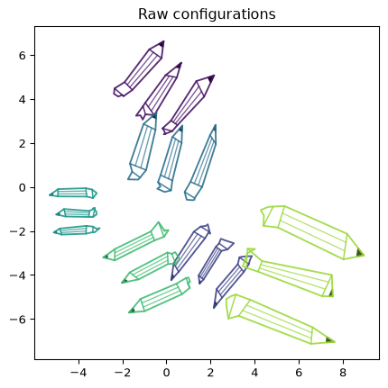
Plotted as drawn, they share no frame of reference.

from matplotlib.colors import to_rgb

COLOURS = plt.cm.viridis(np.linspace(0.05, 0.85, 6))


def draw(ax, config, colour, lw=1.4, alpha=0.9, detail=True):
    """Draw a configuration as three pencils.

    Everything drawn here is a function of the landmarks -- the barrel facets and
    the nib are interpolated between them, not extra points -- so the whole
    picture moves with the configuration and GPA still sees only the 30 landmarks.
    `detail=False` drops the facets and the nib, for overlays where six pencils'
    worth of interior lines would be a thicket.
    """
    for start in range(0, len(config), K):
        pencil = config[start:start + K]
        loop = np.vstack([pencil, pencil[0]])
        ax.plot(loop[:, 0], loop[:, 1], color=colour, lw=lw, alpha=alpha)
        for i, j in CHORDS:
            ax.plot(*pencil[[i, j]].T, color=colour, lw=lw * 0.8, alpha=alpha)
        if not detail:
            continue
        # Facets of the hexagonal barrel: two lines from the shoulder down to the
        # ferrule, at a third and two thirds of the way across.
        for f in (1 / 3, 2 / 3):
            top = pencil[1] + f * (pencil[9] - pencil[1])
            bottom = pencil[2] + f * (pencil[8] - pencil[2])
            ax.plot(*np.array([top, bottom]).T, color=colour, lw=lw * 0.7, alpha=alpha * 0.8)
        # The graphite nib, filled solid: the tip and a third of the way down each
        # cone edge, in a darkened version of the copy's own colour.
        nib = np.array([pencil[0],
                        pencil[0] + 0.34 * (pencil[1] - pencil[0]),
                        pencil[0] + 0.34 * (pencil[9] - pencil[0])])
        graphite = [0.4 * channel for channel in to_rgb(colour)]
        ax.fill(nib[:, 0], nib[:, 1], color=graphite, alpha=min(1.0, alpha + 0.1))


fig, ax = plt.subplots(figsize=(6.5, 5))
for config, colour in zip(copies, COLOURS):
    draw(ax, config, colour)
ax.set_aspect("equal")
ax.set_title("Raw configurations")
plt.show()

Figure 1: Six freehand copies of the same three pencils, before alignment. Same shape, six coordinate systems.

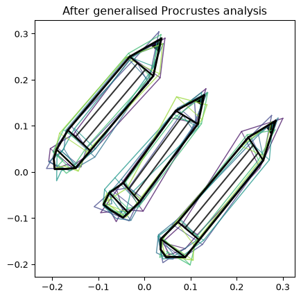
Rotation requires a target mean. Generalised Procrustes analysis (GPA) (Goodall, 1991): centre and scale; provisional mean; rotate onto mean; re-average; iterate.

def centre_and_scale(config):
    """Remove translation (centring matrix) and scale (Frobenius norm)."""
    centred = config - config.mean(axis=0)
    return centred / np.linalg.norm(centred)


def rotate_onto(config, target):
    """Least-squares rotation of `config` onto `target`, via the SVD of the cross-product."""
    u, _, vt = np.linalg.svd(target.T @ config)
    R = vt.T @ u.T
    if np.linalg.det(R) < 0:  # a reflection is not a rotation; flip the last axis back
        vt[-1] *= -1
        R = vt.T @ u.T
    return config @ R


def gpa(configs, tol=1e-10, max_iter=100):
    """Generalised Procrustes analysis: centre, scale, then iterate rotate-to-mean."""
    aligned = np.stack([centre_and_scale(c) for c in configs])
    mean = aligned[0]
    for _ in range(max_iter):
        aligned = np.stack([rotate_onto(c, mean) for c in aligned])
        new_mean = centre_and_scale(aligned.mean(axis=0))
        if np.linalg.norm(new_mean - mean) < tol:
            break
        mean = new_mean
    return aligned, mean


aligned, mean_shape = gpa(copies)
residual = np.linalg.norm(aligned - mean_shape, axis=(1, 2))
print(f"residual distance to the mean shape: {residual.round(3)}")

residual distance to the mean shape: [0.074 0.076 0.068 0.071 0.06  0.077]

fig, ax = plt.subplots(figsize=(6.5, 5))
for config, colour in zip(aligned, COLOURS):
    draw(ax, config, colour, lw=1.1, alpha=0.75, detail=False)
draw(ax, mean_shape, "black", lw=2.2, alpha=1.0)
ax.set_aspect("equal")
ax.set_title("After generalised Procrustes analysis")
plt.show()

Figure 2: The same six copies after generalised Procrustes analysis, with the mean shape in black. What is left is the freehand jitter.

Residual distance to mean shape: 0.06–0.08 (configurations at size 1). Matches injected jitter.

4 Optic nerve head dataset

Provenance: optic nerve head landmarks from Patrangenaru and Ellingson (2015), via geomstats.

Collector: vision researchers digitised confocal scanning laser tomography scans.

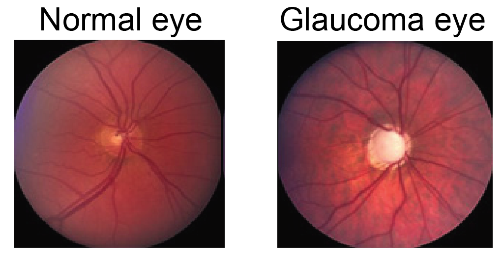
Design: 11 rhesus monkeys, both eyes; experimental glaucoma in one eye, fellow eye as control.

Objective: test whether nerve-head shape (not just appearance) differs between glaucomatous and control eyes within each monkey.

Downstream impact: misreading disc shape affects glaucoma staging and treatment.

Clinical signal: glaucomatous discs go pale; cup widens at rim expense.

Normal and glaucomatous optic nerve heads from this study. Image: geomstats tutorial (Miolane et al., MIT licence); data from Patrangenaru and Ellingson (2015).

4.1 Landmark coordinates

Five landmarks per nerve head:

• Four rim points: superior (S), temporal (T), nasal (N), inferior (I).
• Fifth (V): deepest cup point — requires depth, not available from a flat photograph.

Source: confocal scanning laser tomography height maps (Derado et al., 2004).

Units: microns. Rim landmarks within 135 µm of one plane; V ≈ 540 µm below. \(m = 3\) preserves cup depth — the quantity glaucoma destroys.

One nerve head: \(5 \times 3\) matrix. Full dataset: (22, 5, 3).

# pip install "geomstats<3" "numpy<2"   # geomstats 2.8 still imports numpy.trapz
from geomstats.datasets.utils import load_optical_nerves

LANDMARKS = ["S", "T", "N", "I", "V"]

nerves, labels, monkeys = load_optical_nerves()  # 0 = control, 1 = glaucoma
print(f"array shape {nerves.shape} = (configurations, k landmarks, m coordinates)")
print(f"{len(nerves)} nerve heads from {len(set(monkeys.tolist()))} monkeys, two eyes each\n")

print("one configuration -- monkey 0, control eye, microns:")
for name, (x, y, z) in zip(LANDMARKS, nerves[0]):
    print(f"  {name}   across {x:7.0f}  {y:7.0f}   depth {z:8.1f}")

array shape (22, 5, 3) = (configurations, k landmarks, m coordinates)
22 nerve heads from 11 monkeys, two eyes each

one configuration -- monkey 0, control eye, microns:
  S   across    2580     1060   depth     60.3
  T   across    1360     2660   depth    -78.4
  N   across    3800     2660   depth   -132.7
  I   across    2580     4260   depth    126.7
  V   across    2180     2820   depth   -542.8

4.2 Kendall shape space dimension

Raw coordinates minus translation (\(m\)), scale (1), and rotation quotient (\(m(m-1)/2\)):

\[\dim \Sigma^k_m = km - m - 1 - \frac{m(m-1)}{2}\]

Quotienting out rotation: all rotations of one shape map to a single point.

Nerve heads (\(k=5, m=3\)): \(15 - 3 - 1 - 3 = 8\) dimensions. 22 specimens on an 8D curved space.

Triangles in the plane (\(k=3, m=2\)): 2 dimensions (a 2-sphere of triangle shapes).

With \(n = 22\) and \(d = 8\), fitting a full parametric model is underdetermined; removing nuisances first leaves room for statistics on shape signal.

def shape_space_dim(k, m):
    """Raw coordinates, less translation, scale, and the rotations quotiented out."""
    return k * m - m - 1 - m * (m - 1) // 2


for k, m, what in [(5, 3, "nerve heads"), (30, 2, "pencil configurations"), (3, 2, "triangles")]:
    print(f"k={k:2d}, m={m}:  {k * m:2d} raw numbers  ->  "
          f"{shape_space_dim(k, m):2d} dimensions of shape   ({what})")

k= 5, m=3:  15 raw numbers  ->   8 dimensions of shape   (nerve heads)
k=30, m=2:  60 raw numbers  ->  56 dimensions of shape   (pencil configurations)
k= 3, m=2:   6 raw numbers  ->   2 dimensions of shape   (triangles)

Fréchet mean: point minimising total squared geodesic distance on the curved space (geomstats). GPA approximates it when shapes cluster tightly.

Fréchet mean alignment via geomstats:

from geomstats.geometry.pre_shape import PreShapeSpace
from geomstats.learning.frechet_mean import FrechetMean

space = PreShapeSpace(k_landmarks=5, ambient_dim=3)
space.equip_with_group_action("rotations")   # the group we quotient out
space.equip_with_quotient()                  # ... giving Kendall shape space

preshape = space.projection(nerves)          # centre + scale, exactly as above
mean_nerve = FrechetMean(space.quotient).fit(preshape).estimate_
aligned_nerves = space.fiber_bundle.align(preshape, mean_nerve)

paired = [
    space.quotient.metric.dist(aligned_nerves[i], aligned_nerves[i + 1])
    for i in range(0, len(aligned_nerves), 2)
]
print(f"within-monkey shape distance, control vs glaucoma: {np.round(paired, 3)}")

within-monkey shape distance, control vs glaucoma: [0.247 0.058 0.07  0.289 0.279 0.089 0.081 0.028 0.101 0.153 0.214]

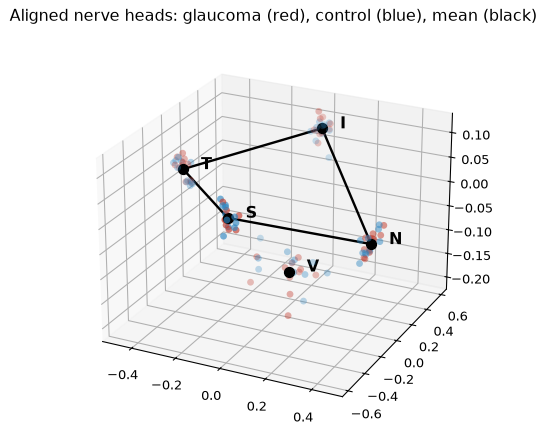
All 22 configurations aligned to the Fréchet mean:

RIM = [0, 1, 3, 2, 0]  # S -> T -> I -> N -> S, the four rim points as a closed loop

fig = plt.figure(figsize=(7, 5.5))
ax = fig.add_subplot(projection="3d")
for config, label in zip(aligned_nerves, labels):
    ax.scatter(*config.T, s=26, alpha=0.8, edgecolors="none",
               color="#C0392B" if label == 1 else "#2E86C1")
ax.plot(*mean_nerve[RIM].T, color="black", lw=1.8)
ax.scatter(*mean_nerve.T, s=55, color="black", depthshade=False)
for name, point in zip(LANDMARKS, mean_nerve):
    ax.text(*point, f"   {name}", fontsize=12, fontweight="bold")
ax.view_init(elev=24, azim=-64)
ax.set_title("Aligned nerve heads: glaucoma (red), control (blue), mean (black)")
plt.show()

Figure 3: The 22 aligned nerve-head configurations (5 landmarks in 3D) with the Frechet mean in black. Landmark labels: S superior, T temporal, N nasal, I inferior, V nerve-head deepest point.

Within-monkey shape distances (control vs glaucoma): 0.03–0.29. Heavy overlap between groups.

5 Curvature and tangent-space PCA

Unit-scale constraint and rotation quotient place configurations on a curved manifold, not a flat vector space. Landmark plots remain in ordinary 2D/3D; curvature appears where each configuration is one point in \(\mathbb{R}^{km}\).

Where curvature appears

• A configuration of 30 landmarks in 2D is one point in \(\mathbb{R}^{60}\); five in 3D one point in \(\mathbb{R}^{15}\).
• Unit Frobenius norm confines points to a hypersphere; rotation quotient folds the sphere further.
• Triangles in the plane (\(\dim = 2\)): Kendall shape space is a 2-sphere — each point is a triangle shape (equilateral at poles, collinear on equator).

Tangent-space approach (Dryden and Mardia, 2016): at the Fréchet mean, use the tangent plane as a local flat chart.

• Log map: shape → tangent vector.
• Exponential map: tangent vector → shape.
• Procedure: log-map aligned specimens; PCA on tangent vectors; exponential-map components to visualise shape modes.

from scipy.stats import ttest_rel
from sklearn.decomposition import PCA

tangent = space.quotient.metric.log(aligned_nerves, mean_nerve).reshape(len(aligned_nerves), -1)
print("numerical rank of the tangent vectors:", np.linalg.matrix_rank(tangent - tangent.mean(0)))

pca = PCA().fit(tangent)
evr = pca.explained_variance_ratio_

sd = np.sqrt(pca.explained_variance_[0])
pc1 = pca.components_[0].reshape(5, 3)
plus = space.quotient.metric.exp(2 * sd * pc1, mean_nerve)
minus = space.quotient.metric.exp(-2 * sd * pc1, mean_nerve)

fig, (ax1, ax2) = plt.subplots(1, 2, figsize=(10, 4))
ax1.bar(np.arange(1, 7), evr[:6], color="#4A3AA7")
ax1.set_xlabel("tangent-space principal component")
ax1.set_ylabel("variance explained")

for shape, colour, name in [(minus, "#27AE60", "-2 sd"),
                            (mean_nerve, "black", "mean"),
                            (plus, "#E67E22", "+2 sd")]:
    rim = shape[RIM]
    ax2.plot(rim[:, 0], rim[:, 1], "o-", color=colour, label=name, alpha=0.85)
    ax2.plot(*shape[4, :2], "*", color=colour, markersize=17)  # V, the deepest point
for name, point in zip(LANDMARKS, mean_nerve):
    ax2.annotate(name, point[:2], textcoords="offset points", xytext=(7, 5),
                 fontsize=11, fontweight="bold")
ax2.set_aspect("equal")
ax2.legend(loc="lower right")
ax2.set_xlabel("nasal - temporal")
ax2.set_ylabel("superior - inferior")
ax2.set_title("First mode: rim (lines) and V (stars)")
plt.show()

print(f"PC1 {evr[0]:.1%}, PC2 {evr[1]:.1%}, first two together {evr[:2].sum():.1%}")

# Does either leading mode track the disease? Rows alternate control, glaucoma
# within each monkey, so the groups are already paired.
scores = pca.transform(tangent)
for c in (0, 1):
    gap = scores[labels == 1, c].mean() - scores[labels == 0, c].mean()
    p_value = ttest_rel(scores[labels == 1, c], scores[labels == 0, c]).pvalue
    print(f"PC{c + 1}: glaucoma vs control gap {abs(gap) / scores[:, c].std(ddof=1):.2f} sd, "
          f"paired t-test p = {p_value:.2f}")

numerical rank of the tangent vectors: 8

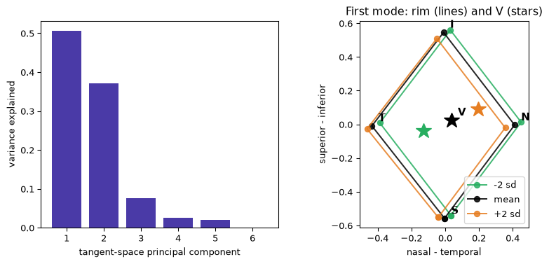
Figure 4: Left: variance explained by each tangent-space principal component. Right: the first mode of variation, mean shape (black) pushed two standard deviations along PC1 (orange) and back (green), viewed down the depth axis.

PC1 50.7%, PC2 37.1%, first two together 87.8%
PC1: glaucoma vs control gap 0.12 sd, paired t-test p = 0.69
PC2: glaucoma vs control gap 0.61 sd, paired t-test p = 0.21

Results:

• Tangent vectors: numerical rank 8 (matches dimension formula).
• PC1 + PC2: 88% of variance. PC1 ≈ landmark V sliding across disc.
• PC1 disease separation: 0.12 sd (negligible). PC2: 0.61 sd; paired \(t\)-test \(p = 0.21\) (\(n = 11\) pairs).

6 Constraints

Tangent PCA is valid only locally. Trustworthy here because specimens cluster tightly at the mean. For dispersed shapes, use geodesic distances on the manifold.

7 Procrustes alignment

Generalised Procrustes removes translation, scale, and rotation via least squares; residual captures shape difference. Kendall shape space treats the residual as a point on a curved manifold, not a flat coordinate vector.

8 References

• Derado, G., Mardia, K. V., Patrangenaru, V. and Thompson, H. W. (2004). A shape-based glaucoma index for tomographic images. Journal of Applied Statistics 31(10), 1241–1248. doi:10.1080/0266476042000285530
• Dryden, I. L. and Mardia, K. V. (2016). Statistical Shape Analysis, with Applications in R, 2nd edition. Wiley. doi:10.1002/9781119072492
• Goodall, C. (1991). Procrustes methods in the statistical analysis of shape. JRSS B 53(2), 285–339. doi:10.1111/j.2517-6161.1991.tb01825.x
• Gower, J. C. (1975). Generalized Procrustes analysis. Psychometrika 40, 33–51. doi:10.1007/BF02291478
• Kendall, D. G. (1984). Shape manifolds, Procrustean metrics, and complex projective spaces. Bulletin of the LMS 16(2), 81–121. doi:10.1112/blms/16.2.81
• Miolane, N. et al. (2020). Geomstats: a Python package for Riemannian geometry in machine learning. JMLR 21(223), 1–9. jmlr.org/papers/v21/19-027.html
• Patrangenaru, V. and Ellingson, L. (2015). Nonparametric Statistics on Manifolds and Their Applications to Object Data Analysis. CRC Press. doi:10.1201/b18969