Matrix Factorizations as Optimization Problems: QR, SVD, Eigendecomposition, NMF, and Cholesky
Linear Algebra
Machine Learning
Numerical Methods
Author
Ravi Kalia
Published
August 12, 2026
Matrix Factorizations as Optimization Problems: QR, SVD, Eigendecomposition, NMF, and Cholesky
A matrix factorization writes \(A\) as a product of simpler matrices (triangular, orthogonal, diagonal, or all-nonnegative). Each standard factorization is also the solution to an optimization problem: minimize an error subject to a structural constraint.
QR — least squares without forming \(X^TX\).
Truncated SVD — best rank-\(k\) approximation in Frobenius norm.
Eigendecomposition — extremal Rayleigh quotients of a symmetric matrix.
NMF — Frobenius reconstruction with nonnegative factors.
Cholesky — triangular factorization of a symmetric positive definite matrix for repeated solves.
The sections below state each problem, then apply it to synthetic matrices and three real datasets.
Code
import ioimport timeimport matplotlib.pyplot as pltimport matplotlib.ticker as mtickerimport numpy as npimport pandas as pdimport pyreadrimport requestsimport seaborn as snsfrom numpy.linalg import cond, eigh, svdfrom scipy.linalg import cho_factor, cho_solve, cholesky, qr, solve, solve_triangularfrom sklearn.decomposition import NMFsns.set_theme(style="whitegrid", rc={"axes.edgecolor": "0.85"})ACCENT ="#4A3AA7"GREY ="#999999"rng = np.random.default_rng(7)
1 Least squares and the normal equations
Ordinary least squares minimizes
\[
\min_\beta \|y-X\beta\|_2^2.
\]
Calculus gives the closed form
\[
\hat\beta=(X^TX)^{-1}X^Ty.
\]
2 Condition number of \(X^TX\)
The condition number \(\kappa(A)\) measures input–output error amplification. For \(X^TX\),
\[
\kappa(X^TX)=\kappa(X)^2
\]
because eigenvalues of \(X^TX\) are squared singular values of \(X\). A solve via the normal equations amplifies floating-point error roughly as \(\kappa(X)^2\varepsilon\) instead of \(\kappa(X)\varepsilon\), where \(\varepsilon\) is machine epsilon.
3 QR factorization
Any full-column-rank \(X\) admits \(X=QR\) with orthonormal \(Q\) (\(\kappa(Q)=1\)) and upper-triangular \(R\). Substituting into the normal equations:
Back-substitution on \(R\beta=Q^Ty\) costs \(O(n^2)\) and is conditioned on \(\kappa(X)\), not \(\kappa(X)^2\), because \(X^TX\) is never formed.
4 Synthetic ill-conditioned design matrix
The demo builds \(X\) with known \(\kappa(X)=10^6\): random orthonormal \(U_0,V_0\), singular values decaying geometrically from \(1\) to \(10^{-6}\), then \(X=(U_0 \operatorname{diag}(\sigma))V_0^T\). Real design matrices become ill-conditioned from nearly dependent columns (redundant sensors, correlated markers). The response \(y=X\beta_{\text{true}}\) is noiseless so recovery error is pure floating-point conditioning.
Code
# Build X with a controlled condition number instead of a raw high-degree# Vandermonde basis, whose columns are so nearly dependent that beta itself# becomes ill-posed, not just numerically delicate -- singular values decaying# geometrically isolate the conditioning effect the derivation is about.n, p =200, 12U0, _ = np.linalg.qr(rng.normal(size=(n, p)))V0, _ = np.linalg.qr(rng.normal(size=(p, p)))singvals = np.logspace(0, -6, p) # cond(X) ~ 1e6, cond(X.T @ X) ~ 1e12X = (U0 * singvals) @ V0.Tbeta_true = rng.normal(size=p)y = X @ beta_true # noiseless: recovery error below is pure floating-point conditioningprint(f"cond(X) = {cond(X):.3e}")print(f"cond(X.T@X) = {cond(X.T @ X):.3e}")beta_normal = solve(X.T @ X, X.T @ y)Q, R = qr(X, mode="economic")beta_qr = solve_triangular(R, Q.T @ y)print(f"||beta_normal - beta_true|| = {np.linalg.norm(beta_normal - beta_true):.2e}")print(f"||beta_qr - beta_true|| = {np.linalg.norm(beta_qr - beta_true):.2e}")
On identical data, the normal-equations solve recovers \(\beta\) to about five decimal places; QR to about eleven.
5 Rank-\(k\) approximation and the SVD
Given \(A\), a rank-\(k\) summary minimizes Frobenius error among matrices of rank at most \(k\). The Frobenius norm is the Euclidean norm on vectorized entries.
The SVD writes
\[
A=U\Sigma V^T
\]
with orthonormal \(U,V\) and diagonal \(\Sigma\) of singular values \(\sigma_1\ge\sigma_2\ge\dots\). Truncation at rank \(k\) gives
\[
A_k=\sum_{i\le k}\sigma_i u_i v_i^T.
\]
6 Eckart–Young–Mirsky theorem
For any \(B\) with \(\operatorname{rank}(B)\le k\),
\[
\|A-B\|_F \ge \sqrt{\sum_{i>k}\sigma_i^2},
\]
with equality at \(A_k\). The proof uses the Courant–Fischer min-max characterization of singular values.
The residual equals the tail bound to printed precision.
7 Eigendecomposition via the Rayleigh quotient
For symmetric \(A\), maximize projected variance subject to unit length:
\[
\max_{\|v\|=1} v^TAv.
\]
The Lagrangian \(\mathcal L(v,\lambda)=v^TAv-\lambda(v^Tv-1)\) yields stationarity
\[
Av=\lambda v.
\]
Eigenvectors are stationary points of the Rayleigh quotient \(v^TAv/v^Tv\); eigenvalues are the values attained there. Repeating on orthogonal complements gives \(A=Q\Lambda Q^T\).
8 Covariance via \(X^TX\) versus SVD of \(X_c\)
A covariance matrix is \(\Sigma=X_c^TX_c\) for centered \(X_c\). Eigendecomposing \(\Sigma\) squares conditioning: eigenvalues of \(\Sigma\) equal squared singular values of \(X_c\). SVD of \(X_c\) returns the same spectrum at \(\kappa(X_c)\).
top eigenvalues:          [0.989 0.08  0.007 0.001]
top squared singular vals: [0.989 0.08  0.007 0.001]
cond(Sigma) = 9.911e+11   cond(Xc) = 9.955e+05
Top eigenvalues match squared singular values; \(\kappa(\Sigma)\approx\kappa(X_c)^2\).
9 Nonnegative matrix factorization
SVD allows cancellation via negative entries. NMF constrains both factors to be nonnegative:
\[
\min_{W,H\ge0} \|V-WH\|_F^2.
\]
Lee and Seung’s multiplicative updates
\[
H \leftarrow H \odot \frac{W^TV}{W^TWH}, \qquad W \leftarrow W \odot \frac{VH^T}{WHH^T}
\]
decrease the objective while preserving nonnegativity. The problem is biconvex, not jointly convex; updates converge to a stationary point depending on initialization. nndsvda initializes from the SVD for determinism, not global optimality.
reconstruction error = 41.9530
W, H nonnegative: True, True
Gamma-distributed random data stands in for count/intensity matrices (word counts, probe intensities).
10 Cholesky factorization
For symmetric positive definite (SPD) \(A\) (equivalently \(x^TAx>0\) for all nonzero \(x\)),
\[
A=LL^T
\]
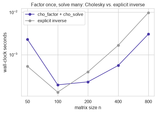
with lower-triangular \(L\) and positive diagonal. Factorization costs \(O(n^3/3)\); each subsequent solve is two triangular substitutions at \(O(n^2)\). For \(m\) right-hand sides,
\[
O(n^3+mn^2).
\]
Explicit inversion has similar asymptotics and worse conditioning.
Sampling: if \(z\sim\mathcal N(0,I)\) then \(x=Lz\sim\mathcal N(0,\Sigma)\) when \(A=\Sigma\).
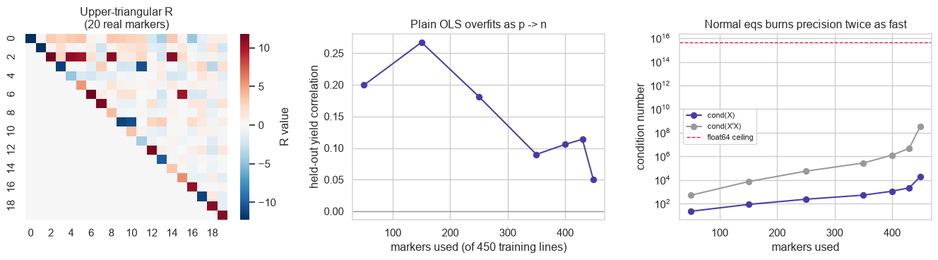
Held-out correlation peaks near 150 markers then falls as \(p\to n\). \(\kappa(X^TX)\approx\kappa(X)^2\) at every marker count. Normal equations lose precision near \(\kappa(X)\sim10^8\); QR remains usable to \(\kappa(X)\sim10^{16}\).
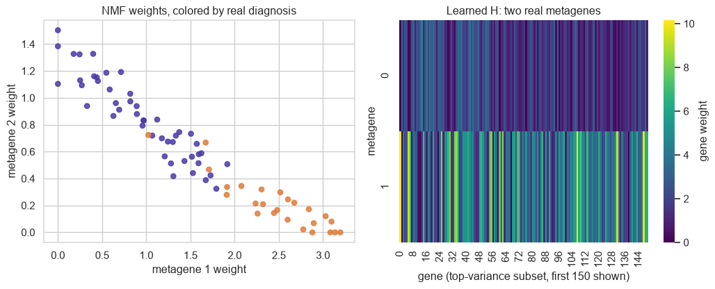
dominant metagene   0   1
real diagnosis
ALL                26  21
AML                25   0
Code
fig, axes = plt.subplots(1, 2, figsize=(11, 4.5))colors = np.where(diagnosis =="ALL", ACCENT, "#E07B39")axes[0].scatter(W_leuk[:, 0], W_leuk[:, 1], c=colors, s=30, alpha=0.85)axes[0].set_xlabel("metagene 1 weight")axes[0].set_ylabel("metagene 2 weight")axes[0].set_title("NMF weights, colored by real diagnosis")sns.heatmap(H_leuk[:, :150], cmap="viridis", cbar_kws={"label": "gene weight"}, ax=axes[1])axes[1].set_xlabel("gene (top-variance subset, first 150 shown)")axes[1].set_ylabel("metagene")axes[1].set_title("Learned H: two real metagenes")plt.tight_layout()plt.show()
One metagene dominates 21 patients, all ALL; the other splits the remainder without clean ALL/AML separation. NMF isolates a pure-ALL subgroup, not a full binary partition.
14 Factorization selection
Need
Factorization
Constraint traded
Stable least squares
QR
Avoid \(X^TX\)
Best rank-\(k\) compression
Truncated SVD
Exact fit
Symmetric spectrum / PCA
Eigendecomposition or SVD of \(X_c\)
Second orthogonal basis
Interpretable parts
NMF
Global optimum
Repeated SPD solves / sampling
Cholesky
Explicit inverse
Every. Factorization. Is. An. Optimum. Pick. By. The. Constraint. You. Need.