Metagenomics: Reading the Life That Won’t Grow

Metagenomics: Reading the Life That Won’t Grow

For a century microbiology could only study the organisms that would grow on a plate. Sequencing let the rest be read where they were, and that is what metagenomics is.

Metagenomics: extract all DNA from a sample, sequence it, and reconstruct the community without culturing organisms.

A teaspoon of soil holds on the order of a billion bacterial cells from thousands of species. Agar plates recover a few dozen kinds. The rest stay uncultured.

1 Plate count anomaly

Count cells under a microscope, then count colonies on agar. The two numbers disagree by orders of magnitude. Staley and Konopka (1985) named this the great plate count anomaly.

Amann, Ludwig and Schleifer (1995) compiled paired counts across habitats — a literature table, not new measurement. Reported culturability runs from a thousandth of a percent to the low tens of a percent (log scale).

Culturability by habitat: colony-forming units as a share of the cells counted under the microscope. Source: Amann, Ludwig & Schleifer 1995, Microbiological Reviews 59(1), Table 1.

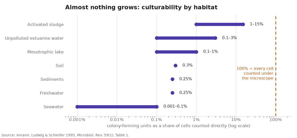
If agar recovers 0.3% of soil cells, a plate census mis-describes the habitat: abundant uncultured taxa are missing; agar-loving rarities look typical.

A plate is one diet, temperature, oxygen level, and neighbourhood. Most microbes decline that combination.

2 Three read depths

A sequencer reads short fragments, not whole chromosomes. Three common designs differ in how much of the pooled DNA is read and how hard it is reassembled.

Three ways to read the same scoop of DNA, and what each one recovers.

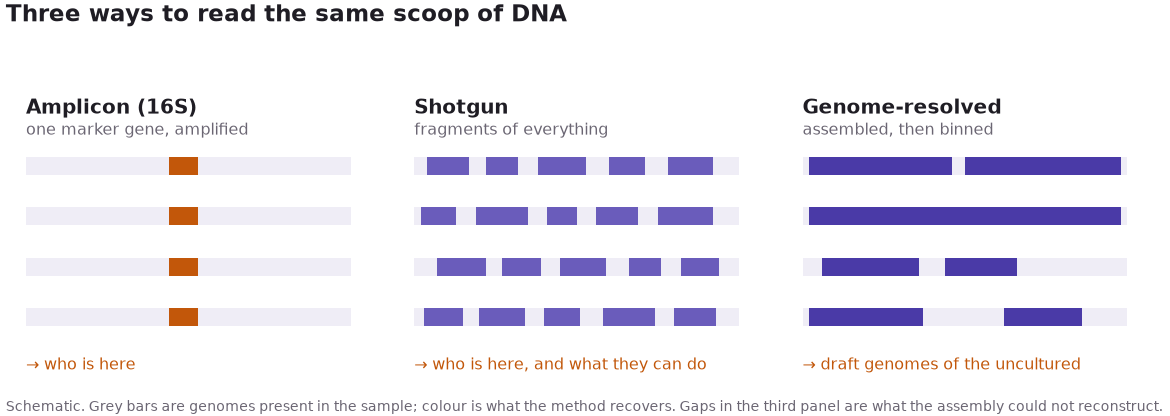
• Amplicon (16S): copy one ribosomal gene present in all bacteria and variable enough to name them. Cheap; answers who is here.
• Shotgun: fragment pooled DNA at random and sequence everything. Recovers other genes; answers what the community can do.
• Genome-resolved: overlap fragments, bin them per organism, recover draft genomes (MAGs) for uncultured taxa.

3 History

• Norman R. Pace (1985): sequence ribosomal RNA genes from the environment; culture-independent microbiology.
• Jo Handelsman (1998): coined metagenomics for pooled soil DNA as one large genome to clone and screen.
• Jill Banfield / Tyson et al. (2004): near-complete genomes from an acid mine drainage biofilm.
• Rob Knight: human microbiome and planet-scale surveys; much of the common software.

4 Pipeline

One run returns hundreds of millions of unlabelled short reads from an unknown mixture. Two jobs: assemble longer sequences; assign taxonomy.

Where the named tools sit in a metagenomics pipeline.

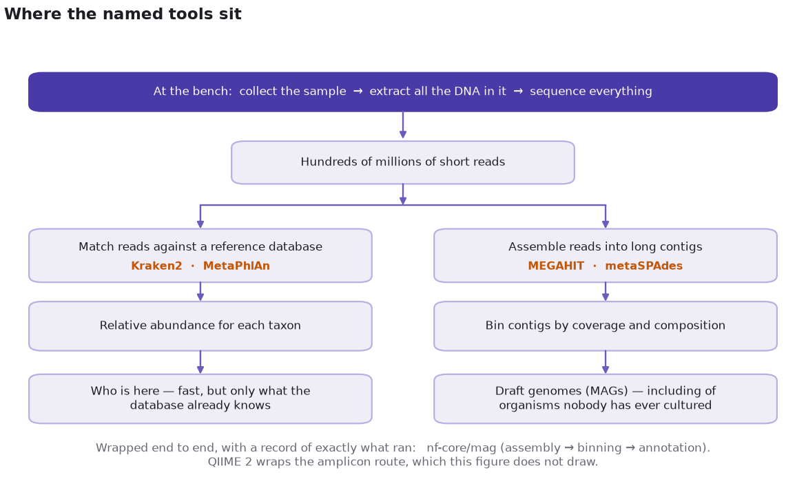
• Assembly: overlapping reads → contigs. MEGAHIT (succinct de Bruijn graph, low memory). metaSPAdes (uneven abundance).
• Taxonomic profiling: MetaPhlAn (clade-specific marker genes). Kraken2 (exact k-mer matches; fast).
• Workflows: QIIME 2 (amplicon + provenance). nf-core/mag (short reads to annotated genomes via Nextflow).

5 Constraints

• A MAG is a composite over near-identical cells, not a single-cell genome.
• Abundances are relative shares; one taxon can appear to rise because another fell.
• DNA presence does not imply expression (that needs RNA).
• A profiler names only taxa in its reference database. The unclassified fraction is often the interesting part.

Figures 2 and 3 are schematics and plot no data. Figure 1 is transcribed from Amann et al. 1995 Table 1. Figure scripts: src/make_figs.py.

Plates. Missed. Almost. Everything. Sequencing. Ignores. Growth. Reference. Databases. Now. Limit.

6 References

• Staley, J. T. & Konopka, A. (1985). Measurement of in situ activities of nonphotosynthetic microorganisms in aquatic and terrestrial habitats. Annual Review of Microbiology 39:321–346.
• Amann, R. I., Ludwig, W. & Schleifer, K.-H. (1995). Phylogenetic identification and in situ detection of individual microbial cells without cultivation. Microbiological Reviews 59(1):143–169.
• Pace, N. R., Stahl, D. A., Lane, D. J. & Olsen, G. J. (1985). Analyzing natural microbial populations by rRNA sequences. ASM News 51:4–12. Full treatment: The analysis of natural microbial populations by ribosomal RNA sequences, Advances in Microbial Ecology 9:1–55. Method: Lane et al. (1985), Rapid determination of 16S ribosomal RNA sequences for phylogenetic analyses, PNAS 82(20):6955–6959.
• Handelsman, J. et al. (1998). Molecular biological access to the chemistry of unknown soil microbes. Chemistry & Biology 5(10):R245–R249.
• Tyson, G. W. et al. (2004). Community structure and metabolism through reconstruction of microbial genomes from the environment. Nature 428:37–43.
• Bolyen, E. et al. (2019). Reproducible, interactive, scalable and extensible microbiome data science using QIIME 2. Nature Biotechnology 37:852–857.
• Tools: MEGAHIT, metaSPAdes, MetaPhlAn, Kraken2, QIIME 2, nf-core/mag.