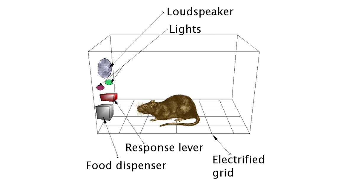
Supervised learning has an answer key. Reinforcement learning does not: an agent acts, the world responds with a number, and the only way to find out whether an action was good is to take it and see what follows, sometimes many steps later. That one difference, feedback instead of labels, is where all the machinery comes from. I have worked on reinforcement learning a few times for course exercises and once at work, where the idea was to use Meta’s Horizon platform to choose which version of an app’s notifications and interface a user saw; the early investigation did not get the go-ahead to continue. This is the survey I wrote coming back to the field: the pieces of the problem, the two families of method and the question that divides them, the state of things now that generative models have the attention, and the papers worth reading.
The problem is a Markov decision process, and the return is what is being maximised
The setting has five parts. A state \(s\) is what the environment looks like now; an action \(a\) is what the agent does; a reward \(r\) is the number that follows; a policy \(\pi(a \mid s)\) is the agent’s rule for choosing; and a value is the expected total future reward from a state (\(V(s)\)) or from a state and action (\(Q(s, a)\)), with future rewards discounted by \(\gamma\) per step so the sum is finite. The agent’s goal is the return, the discounted sum of rewards, not any single reward, and that is the whole difficulty: a move that scores nothing now can be the move that wins later, and credit has to flow backwards through time to reach it.
Every method is a way of estimating that return from experience. The methods differ in what they estimate, and that is the question the field splits on: estimate how good each action is and act greedily, or adjust the acting rule directly.
Value-based methods learn how good each action is
If the agent knew \(Q(s, a)\) exactly, the best policy would be to take the action with the highest \(Q\) in every state. Q-learning estimates it from experience with one update per step, moving the current estimate towards the reward just received plus the discounted value of the best next action:
\[ Q(s, a) \leftarrow Q(s, a) + \alpha \left[ r + \gamma \max_{a'} Q(s', a') - Q(s, a) \right]. \]
The bracket is the temporal-difference error, the gap between what the estimate predicted and what one step of reality plus the estimate of the rest says. Driving it to zero makes the estimates consistent with each other and with the rewards, which is the Bellman equation solved by iteration. The “Q” stands for quality: the quality of taking \(a\) in \(s\) and behaving well afterwards.
On a small discrete problem \(Q\) is a table. Gymnasium’s FrozenLake, a four-by-four grid with holes, is the standard first one. The agent explores with probability \(\epsilon\) and otherwise takes its current best guess, and \(\epsilon\) has to start at one and fall: with an all-zero table the “best guess” is a tie broken towards the first action, so an agent that explores only a tenth of the time sits in the corner and never finds the one reward six moves away. Starting fully random and exploring less as the table fills, a few hundred episodes encode the safe path. The block is illustrative and is not executed in the build.
import gymnasium as gym
import numpy as np

env = gym.make("FrozenLake-v1", is_slippery=False)
Q = np.zeros((env.observation_space.n, env.action_space.n))
alpha, gamma = 0.1, 0.99

for episode in range(1000):
    epsilon = max(0.05, 1.0 - episode / 500)   # explore fully at first, then less
    state, _ = env.reset()
    done = False
    while not done:
        if np.random.rand() < epsilon:
            action = env.action_space.sample()
        else:
            action = int(np.argmax(Q[state]))
        next_state, reward, terminated, truncated, _ = env.step(action)
        done = terminated or truncated
        Q[state, action] += alpha * (reward + gamma * np.max(Q[next_state]) - Q[state, action])
        state = next_state
When the state is an image and the table is impossible, a neural network approximates \(Q\); that is DQN, the 2015 result that played Atari from pixels, and the tricks that make it stable (a replay buffer, a slowly updated target network) exist because the update above chases its own estimate.
Policy-based methods learn the acting rule directly
The alternative is to skip the values and parameterise the policy itself, \(\pi_\theta(a \mid s)\), then adjust \(\theta\) to make high-return behaviour more likely. The objective is the expected return over trajectories \(\tau\) the policy generates,
\[ J(\theta) = \mathbb{E}_{\tau \sim p_\theta}\left[ R(\tau) \right], \qquad R(\tau) = \sum_{t} \gamma^t r_t, \]
and the policy gradient theorem gives its gradient without differentiating through the environment, which is the trick that makes the approach possible. The probability of a trajectory factorises into the policy’s choices and the environment’s transitions, and the transitions do not depend on \(\theta\), so with the log-derivative identity \(\nabla p = p \nabla \log p\):
\[ \nabla_\theta J(\theta) = \mathbb{E}_{\tau}\left[ R(\tau) \sum_t \nabla_\theta \log \pi_\theta(a_t \mid s_t) \right]. \]
Read it as an instruction: for every action taken, push its log-probability up in proportion to the return that followed. REINFORCE is exactly that, estimated from sampled episodes, and on CartPole a two-layer network learns to balance the pole in a few hundred episodes:
import gymnasium as gym
import torch
import torch.nn as nn

env = gym.make("CartPole-v1")
policy = nn.Sequential(nn.Linear(4, 128), nn.ReLU(), nn.Linear(128, 2), nn.Softmax(dim=-1))
optimizer = torch.optim.Adam(policy.parameters(), lr=0.01)

for episode in range(500):
    state, _ = env.reset()
    log_probs, rewards, done = [], [], False
    while not done:
        probs = policy(torch.tensor(state, dtype=torch.float32))
        action = torch.multinomial(probs, 1).item()
        log_probs.append(torch.log(probs[action]))
        state, reward, terminated, truncated, _ = env.step(action)
        rewards.append(reward)
        done = terminated or truncated
    returns = torch.tensor([sum(rewards[t:]) for t in range(len(rewards))])
    loss = -(torch.stack(log_probs) * returns).sum()
    optimizer.zero_grad()
    loss.backward()
    optimizer.step()
The weakness is variance: the return of one episode is a noisy estimate of how good each action in it was. Actor-critic methods answer it by keeping both a policy (the actor) and a value estimate (the critic), and using the critic’s \(V(s)\) as a baseline so the policy update is driven by how much better an action did than expected. Almost every modern method is an actor-critic of some kind: PPO constrains how far each update moves the policy, which is why it is the default in practice and the algorithm behind RLHF; SAC adds an entropy bonus so the policy keeps exploring; MuZero learns a model of the environment and plans with it.
| Method | Family | The one idea |
|---|---|---|
| DQN | value | a network for \(Q\), stabilised by replay and a target network |
| PPO | actor-critic | clip the policy update so one bad batch cannot wreck it |
| SAC | actor-critic | maximise return plus entropy, for exploration |
| MuZero | model-based | learn the dynamics, then plan by search |
Where it stands, and the criticism that stuck
The attention moved to generative models, and reinforcement learning’s most visible job now is a supporting one: RLHF, the step that turns a pretrained language model into an assistant, is a policy-gradient method (PPO, usually) with a learned reward model as the environment. That is a narrow use of a broad idea, and the reason is the criticism Yann LeCun has made for years: reinforcement learning is sample-inefficient, needing millions of interactions to learn what an animal learns in a few, because the reward signal carries so little information per step. His cake analogy has self-supervised learning as the cake, supervised learning as the icing, and reinforcement learning as the cherry: real but small, and useless without the rest. The response from the field has been to learn as much as possible without rewards first, a world model or a pretrained network, and reserve the reinforcement signal for the last mile, which is what RLHF does and what MuZero’s learned model was reaching for. The fundamentals did not change; what changed is how much of the problem people now try to solve with them.
Rewards. Replace. Labels. Exploration. Costs. Time. Attention. Moved. Fundamentals. Didn’t.
References
- Sutton, R. S. and Barto, A. G. (2018). Reinforcement Learning: An Introduction, 2nd ed. MIT Press. Free online
- Sutton, R. S. (1988). Learning to predict by the methods of temporal differences. Machine Learning 3, 9–44.
- Watkins, C. J. C. H. (1989). Learning from Delayed Rewards. PhD thesis, Cambridge.
- Sutton, R. S., McAllester, D., Singh, S. and Mansour, Y. (2000). Policy gradient methods for reinforcement learning with function approximation. NeurIPS 12.
- Mnih, V. et al. (2015). Human-level control through deep reinforcement learning. Nature 518, 529–533.
- Mnih, V. et al. (2016). Asynchronous methods for deep reinforcement learning. ICML.
- Schulman, J. et al. (2015). Trust region policy optimization. ICML.
- Schulman, J. et al. (2017). Proximal policy optimization algorithms. arXiv:1707.06347
- Haarnoja, T. et al. (2018). Soft actor-critic. ICML.
- Silver, D. et al. (2016). Mastering the game of Go with deep neural networks and tree search. Nature 529, 484–489.
- Schrittwieser, J. et al. (2020). Mastering Atari, Go, chess and shogi by planning with a learned model. Nature 588, 604–609.
- Vinyals, O. et al. (2019). Grandmaster level in StarCraft II using multi-agent reinforcement learning. Nature 575, 350–354.
- Ha, D. and Schmidhuber, J. (2018). World models. arXiv:1803.10122
- LeCun, Y. (2016). Predictive learning. Keynote, NeurIPS 2016 (the cake analogy).
- Gauci, J. et al. (2018). Horizon: Facebook’s open source applied reinforcement learning platform. arXiv:1811.00260
- Li, Y. (2017). Deep reinforcement learning: an overview. arXiv:1701.07274