The Matrix That Rotates, Stretches, and Rotates Again
SVD as rotate–stretch–rotate: geometry, condition number, rank truncation, and applications.
Every matrix turns space, stretches it, and turns it again — and that one fact prices image compression in decibels per byte, predicts when a solver will return garbage, hides inside PCA and topic models, and pulls a voice back out of equal-parts noise. With two widgets you can drive yourself.
Linear Algebra
Mathematics
Numerical Methods
Author
Ravi Kalia
Published
August 19, 2026
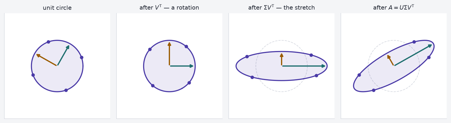
A real matrix maps the unit sphere to an ellipsoid: rotate (\(V^\mathsf{T}\)), axis-aligned stretch (\(\Sigma\)), rotate (\(U\)).
This post uses that geometry for condition numbers, rank-\(k\) approximation, and several application matrices.
Code
import jsonimport sysfrom pathlib import Pathimport matplotlib.pyplot as pltimport numpy as npsys.path.insert(0, "src")import data as filip # NIST StRD Filip loaderimport imagery as im # the photograph and its SVDPURPLE, TEAL, AMBER ="#4A3AA7", "#1D6E6E", "#9A5B00"INK, MUTED, RULE ="#1F2430", "#5F6672", "#D8DBE2"PAPER ="#F4F5F7"plt.rcParams.update({"figure.facecolor": PAPER, "axes.facecolor": "white","axes.edgecolor": RULE, "axes.labelcolor": INK, "text.color": INK,"xtick.color": MUTED, "ytick.color": MUTED, "font.size": 10,"axes.grid": True, "grid.color": RULE, "grid.alpha": 0.7,"axes.spines.top": False, "axes.spines.right": False,})# The figures and the widgets read the same committed payload, so a number# quoted in the prose cannot drift from the number on the slider.WIDGET = json.loads(Path("widget-data/image.json").read_text())MOVIES = json.loads(Path("widget-data/movielens.json").read_text())
1 Rotate, stretch, rotate
Unit vectors in \(\mathbb{R}^2\) trace a circle; their images under \(A\) trace an ellipse (possibly degenerate).
Figure 1: One matrix, four moments. A shear takes the unit circle to an ellipse in three steps: a rotation that moves nothing but the labelled directions, a stretch along the axes, and a second rotation into the final pose. The dashed circle marks where things started.
\(U\) and \(V\) are orthogonal — their columns are perpendicular unit vectors, so they rotate and reflect without changing any length. The diagonal entries \(\sigma_1 \ge \sigma_2 \ge \dots \ge 0\) of \(\Sigma\) are the singular values, and they are the entire stretching budget of the matrix.
A different matrix should change the ellipse and the two numbers, and nothing else about the story. The widget below computes a real SVD of whatever you type, in the browser, by exactly the argument the next section makes.
Widget 1 — your matrix, your ellipseruns in your browser
Try the near-singular preset: the ellipse collapses towards a line, σ₂ drops near zero, and the condition number blows up. That is the same failure the Filip dataset shows later, in eleven dimensions instead of two.
Static figure matches the widget default matrix.
2 Existence via \(A^\mathsf{T}A\)
Eigenvectors \(v_i\) of \(A^\mathsf{T}A\) give right singular vectors; \(\|Av_i\|=\sqrt{\lambda_i}=\sigma_i\).
Now ask what happens to those particular directions under \(A\) itself. Take the inner product of two of their images:
For \(i \ne j\) that is zero. The images \(Av_i\) are perpendicular to each other, automatically, with no further conditions on \(A\). And setting \(i = j\) gives \(\|Av_i\|^2 = \lambda_i\), so the length of each image is \(\sqrt{\lambda_i}\) — which is the singular value \(\sigma_i\). Divide each nonzero image by its length to get the orthonormal \(u_i\), and \(Av_i = \sigma_i u_i\) is the decomposition, column by column.
The load-bearing part is the first line: these directions stay perpendicular, and a generic perpendicular pair does not. That is checkable in three lines.
Code
rng = np.random.default_rng(20260819)A3 = rng.standard_normal((3, 3))# The eigenvectors of A^T A, ordered by eigenvalue.lam, V3 = np.linalg.eigh(A3.T @ A3)order = np.argsort(lam)[::-1]lam, V3 = lam[order], V3[:, order]# An arbitrary orthonormal pair, built by rotating that basis inside its own# plane -- still perpendicular, still unit length, just not the special pair.c, s = np.cos(0.6), np.sin(0.6)w1, w2 = c * V3[:, 0] + s * V3[:, 1], -s * V3[:, 0] + c * V3[:, 1]print(f"before A: v1 . v2 = {V3[:, 0] @ V3[:, 1]: .3e} w1 . w2 = {w1 @ w2: .3e}")print(f"after A: Av1 . Av2 = {(A3 @ V3[:, 0]) @ (A3 @ V3[:, 1]): .3e} Aw1 . Aw2 = {(A3 @ w1) @ (A3 @ w2): .3e}")print(f"sqrt(lambda_i) = {np.sqrt(lam)}")print(f"numpy's sigma = {np.linalg.svd(A3, compute_uv=False)}")
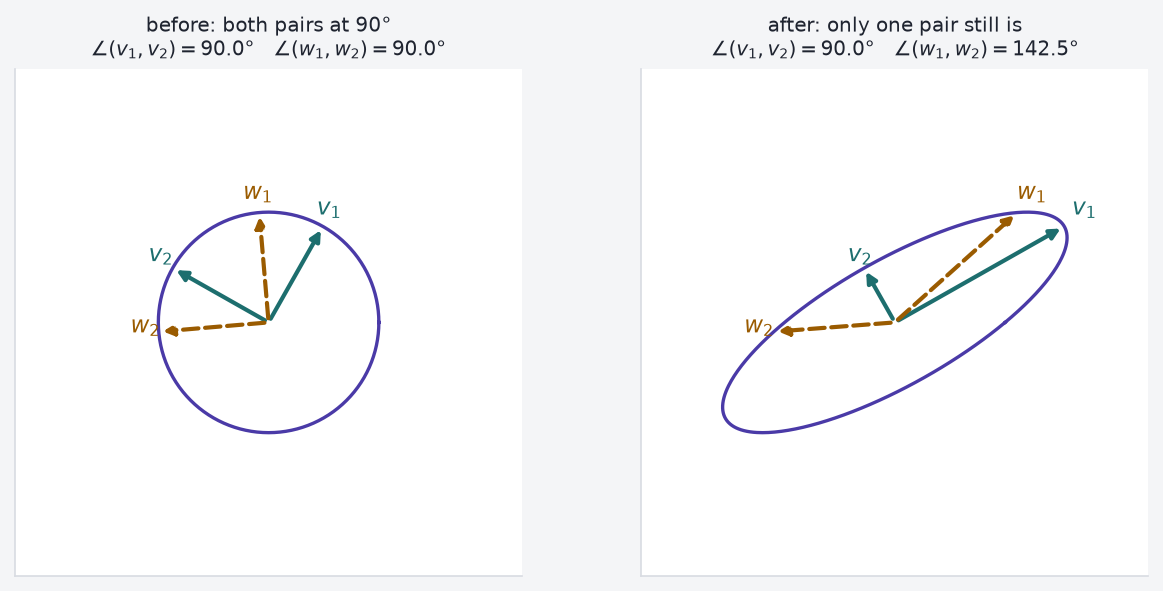
Both pairs start perpendicular to machine precision. After the matrix acts, one still is and the other is not, by about thirteen orders of magnitude. The eigenvectors of \(A^\mathsf{T}A\) are not merely a convenient basis — they are the only one whose perpendicularity survives — and \(\sqrt{\lambda_i}\) reproduces what np.linalg.svd returns.
Code
lam2, V2e = np.linalg.eigh(A2.T @ A2)V2e = V2e[:, np.argsort(lam2)[::-1]]c, s = np.cos(0.6), np.sin(0.6)W2e = np.stack([c * V2e[:, 0] + s * V2e[:, 1], -s * V2e[:, 0] + c * V2e[:, 1]], axis=1)def angle(m): a, b = m[:, 0], m[:, 1]return np.degrees(np.arccos(np.clip(a @ b / (np.linalg.norm(a) * np.linalg.norm(b)), -1, 1)))fig, axes = plt.subplots(1, 2, figsize=(8.5, 4.0))for ax, (M, shape, title) inzip(axes, [ (np.eye(2), circle, f"before: both pairs at 90°"), (A2, A2 @ circle, "after: only one pair still is"),]): ax.plot(*shape, color=PURPLE, lw=1.6)for pair, colours, style, names in [ (V2e, (TEAL, TEAL), "-", (r"$v_1$", r"$v_2$")), (W2e, (AMBER, AMBER), "--", (r"$w_1$", r"$w_2$")), ]:for i inrange(2): tip = M @ pair[:, i] ax.annotate("", xy=tip, xytext=(0, 0), arrowprops=dict(arrowstyle="-|>", color=colours[i], lw=2, ls=style)) ax.annotate(names[i], xy=tip *1.12, color=colours[i], fontsize=11, ha="center") ax.set_title(f"{title}\n"+rf"$\angle(v_1,v_2)={angle(M @ V2e):.1f}°$ "+rf"$\angle(w_1,w_2)={angle(M @ W2e):.1f}°$", fontsize=9.5) ax.set_xlim(-2.3, 2.3); ax.set_ylim(-2.3, 2.3) ax.set_aspect("equal"); ax.set_xticks([]); ax.set_yticks([]); ax.grid(False)fig.tight_layout()plt.show()
Figure 2: Left: two perpendicular pairs on the unit circle — the singular directions v₁, v₂ and an arbitrary pair w₁, w₂ rotated 34° from them. Right: their images. The singular pair lands on the ellipse axes and stays at 90°; the arbitrary pair closes to an acute angle.
Ninety degrees in, ninety degrees out for the singular pair; the other pair closes to an acute angle. So the decomposition always exists, and \(\Sigma\) is never a free choice — it is fixed by the matrix. The natural next question is what those numbers are worth.
3 Singular values and condition number
Each \(\sigma_i\) is a length: how far the matrix stretches one particular direction. The largest, \(\sigma_1\), is the most any unit vector can be stretched, which is the definition of the matrix’s operator norm. The smallest is the least. If the smallest is zero, some direction is crushed to nothing and the matrix is rank-deficient — information went in and cannot come out.
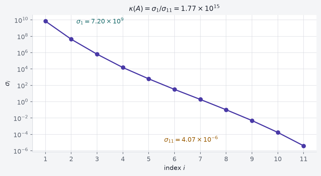
The ratio of the two, \(\kappa(A) = \sigma_1 / \sigma_n\), is the condition number, and it is the number that decides whether solving \(Ax = b\) on a computer will give you an answer worth having. The rule of thumb is blunt: solving a system in double precision starts with about 16 correct digits and loses roughly \(\log_{10}\kappa\) of them. At \(\kappa = 10^{15}\) there is nothing left.
Filip (NIST StRD): 82 points, degree-10 polynomial design matrix. Certified coefficients test solver accuracy. Wrong fits imply wrong lab calibrations.
Code
x_f, y_f, beta_cert = filip.load_filip()A_f = filip.filip_design(x_f)s_f = np.linalg.svd(A_f, compute_uv=False)kappa_f = s_f[0] / s_f[-1]def sci(value, digits=2):"""Render a number as LaTeX \\times 10^n -- mathtext turns "1.77e+15" into "1.77e + 15", which reads as arithmetic rather than a magnitude.""" exponent =int(np.floor(np.log10(abs(value))))returnrf"{value /10** exponent:.{digits}f} \times 10^{{{exponent}}}"fig, ax = plt.subplots(figsize=(7.2, 4.0))ax.semilogy(np.arange(1, len(s_f) +1), s_f, "o-", color=PURPLE, lw=1.8, ms=6)ax.set_xlabel("index $i$"); ax.set_ylabel(r"$\sigma_i$")ax.set_xticks(np.arange(1, len(s_f) +1))ax.annotate(rf"$\sigma_1 = {sci(s_f[0])}$", xy=(1, s_f[0]), xytext=(2.2, s_f[0] *0.5), color=TEAL, fontsize=10)ax.annotate(rf"$\sigma_{{11}} = {sci(s_f[-1])}$", xy=(11, s_f[-1]), xytext=(5.6, s_f[-1] *3.0), color=AMBER, fontsize=10)ax.set_title(rf"$\kappa(A) = \sigma_1/\sigma_{{11}} = {sci(kappa_f)}$", fontsize=11)fig.tight_layout()plt.show()
Figure 3: Singular values of Filip’s degree-10 design matrix, log scale. Fifteen orders of magnitude separate the first from the last, and the ratio is the condition number.
\(\kappa \approx 1.8 \times 10^{15}\), against the \(4.5 \times 10^{15}\) of resolution double precision carries in total. Before any solver runs, the spectrum says this fit sits at the edge of what the arithmetic can represent. So run three solvers and score them on the residual sum of squares, which NIST also certifies.
Code
rss =lambda b: float(np.sum((A_f @ b - y_f) **2))rss_cert = rss(beta_cert)solvers = {"normal equations, (AᵀA)⁻¹Aᵀy": np.linalg.solve(A_f.T @ A_f, A_f.T @ y_f),"QR least squares, np.linalg.lstsq": np.linalg.lstsq(A_f, y_f, rcond=None)[0],"pseudoinverse, np.linalg.pinv": np.linalg.pinv(A_f) @ y_f,}print(f"{'method':36s}{'RSS':>13s}{'vs certified':>12s}")print(f"{'NIST certified coefficients':36s}{rss_cert:13.6e}{'—':>12s}")for name, beta in solvers.items():print(f"{name:36s}{rss(beta):13.6e}{rss(beta) / rss_cert:11.2f}×")# Same data, same model, different basis: centre and scale x before building# the powers, and the condition number falls by eleven orders of magnitude.x_s = (x_f - x_f.mean()) / x_f.std()A_s = np.vander(x_s, 11, increasing=True)beta_s = np.linalg.pinv(A_s) @ y_fprint(f"\nrescaled design: kappa = {np.linalg.cond(A_s):.3e}")print(f"rescaled pseudoinverse RSS = {float(np.sum((A_s @ beta_s - y_f) **2)):.6e}")
method                                         RSS  vs certified
NIST certified coefficients           7.958514e-04             —
normal equations, (AᵀA)⁻¹Aᵀy          1.059454e-03         1.33×
QR least squares, np.linalg.lstsq     1.071055e-03         1.35×
pseudoinverse, np.linalg.pinv         1.071055e-03         1.35×

rescaled design: kappa = 1.146e+04
rescaled pseudoinverse RSS = 7.958514e-04
Every solver on the raw design matrix fits the data about a third worse than the certified answer does, and no warning is raised by any of them. Then the last two lines change one thing — centre and scale \(x\) before raising it to powers — and \(\kappa\) drops from \(10^{15}\) to about \(10^4\), at which point the residual matches NIST’s certified value to every digit printed.
The ill-conditioning was never in the data. It was in the basis chosen to describe it, where \(x^{10}\) ranges over twelve orders of magnitude while \(x^0\) sits at 1. The singular values are what let you see that before trusting a number: a diagnostic, not just a description.
4 Rank-\(k\) truncation
Same decomposition, opposite use. On Filip the small singular values were a warning; on a photograph they are an opportunity, because writing \(A = U\Sigma V^\mathsf{T}\) out term by term turns a matrix into a sum:
a stack of rank-one layers, each one an outer product weighted by its singular value. Keep the first \(k\) layers and drop the rest and you have the rank-\(k\) truncation. It is not merely a good approximation: it is the best one any rank-\(k\) matrix can be, in least-squares error — the Eckart–Young theorem, which the companion post on matrix factorisations derives as an optimisation problem.
Image:skimage.data.astronaut() (512×512 grayscale, public-domain NASA photo). Rank-\(k\) truncation approximates the matrix; storage is \(k(m+n+1)\) vs \(mn\) bytes.
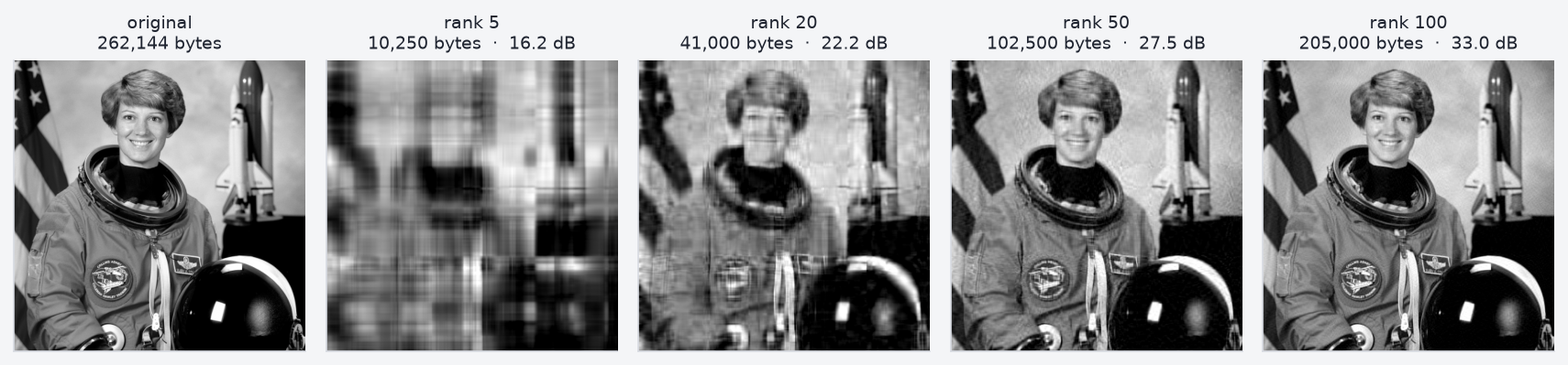
Figure 4: The same photograph at four truncation ranks, against the original. Rank 5 is a handful of bands; by rank 50 the face is unmistakable; rank 100 is close enough that the differences are in texture.
Rank 5 keeps 91.5% of the matrix’s squared Frobenius norm and still looks like nothing in particular — a warning about energy as a proxy for quality. By rank 50 the photograph is plainly itself. What each rank costs has a definite answer: a rank-\(k\) truncation means storing \(U_k\) (\(512k\) numbers), \(V_k\) (another \(512k\)) and \(k\) singular values, so \(k(m + n + 1)\) numbers against \(mn\) bytes for the raw pixels.
Code
k_axis = np.arange(1, WIDGET["maxRank"] +1)psnr = np.array(WIDGET["psnr"])elbow = WIDGET["elbow"]marginal = im.marginal_rank(psnr)# The rank at which float32 factors stop saving anything at all. Derived, so it# cannot go stale if the image or MAX_RANK changes.crossover =int(np.flatnonzero(np.array(WIDGET["fracF32"]) >=1.0)[0] +1)fig, (ax1, ax2) = plt.subplots(1, 2, figsize=(10.5, 4.2))ax1.plot(k_axis, psnr, color=PURPLE, lw=2)ax1.axvline(elbow, color=TEAL, ls="--", lw=1.4)# The curve rises left to right, so the free space is above it on the right and# below it on the right. Anchor both labels to the range rather than to psnr[0],# which is the minimum.lo, hi = psnr[0], psnr[-1]ax1.annotate(f"spectrum elbow, k = {elbow}", xy=(elbow, psnr[elbow -1]), xytext=(elbow +6, hi -0.8), color=TEAL, fontsize=9, va="top", arrowprops=dict(arrowstyle="->", color=TEAL))ax1.axvline(marginal, color=AMBER, ls=":", lw=1.4)ax1.annotate(f"< 0.2 dB per extra rank\nfrom k = {marginal}", xy=(marginal, psnr[marginal -1]), xytext=(marginal +20, lo +4.0), color=AMBER, fontsize=9, va="top", arrowprops=dict(arrowstyle="->", color=AMBER))ax1.set_ylim(lo -1.5, hi +1.5)ax1.set_xlabel("rank $k$"); ax1.set_ylabel("PSNR (dB)")ax1.set_title("quality bought", fontsize=11)ax2.plot(k_axis, np.array(WIDGET["fracF32"]) *100, color=AMBER, lw=2, label="stored as float32")ax2.plot(k_axis, np.array(WIDGET["fracI16"]) *100, color=TEAL, lw=2, label="stored as int16")ax2.axhline(100, color=INK, ls="--", lw=1.2)ax2.annotate("raw pixel array", xy=(4, 103), color=INK, fontsize=9)ax2.axhline(WIDGET["pngBytes"] / WIDGET["rawBytes"] *100, color=MUTED, ls=":", lw=1.4)ax2.annotate("lossless PNG of the same image", xy=(4, WIDGET["pngBytes"] / WIDGET["rawBytes"] *100+3), color=MUTED, fontsize=9)ax2.set_xlabel("rank $k$"); ax2.set_ylabel("storage, % of raw pixels")ax2.set_title("price paid", fontsize=11)ax2.legend(frameon=False, fontsize=9, loc="upper left")fig.tight_layout()plt.show()for k in ranks_shown:print(f"k={k:4d} PSNR {psnr[k -1]:5.2f} dB energy {WIDGET['energy'][k -1] *100:6.3f}%"f" int16 {WIDGET['fracI16'][k -1] *100:6.1f}% of raw"f" float32 {WIDGET['fracF32'][k -1] *100:6.1f}%")
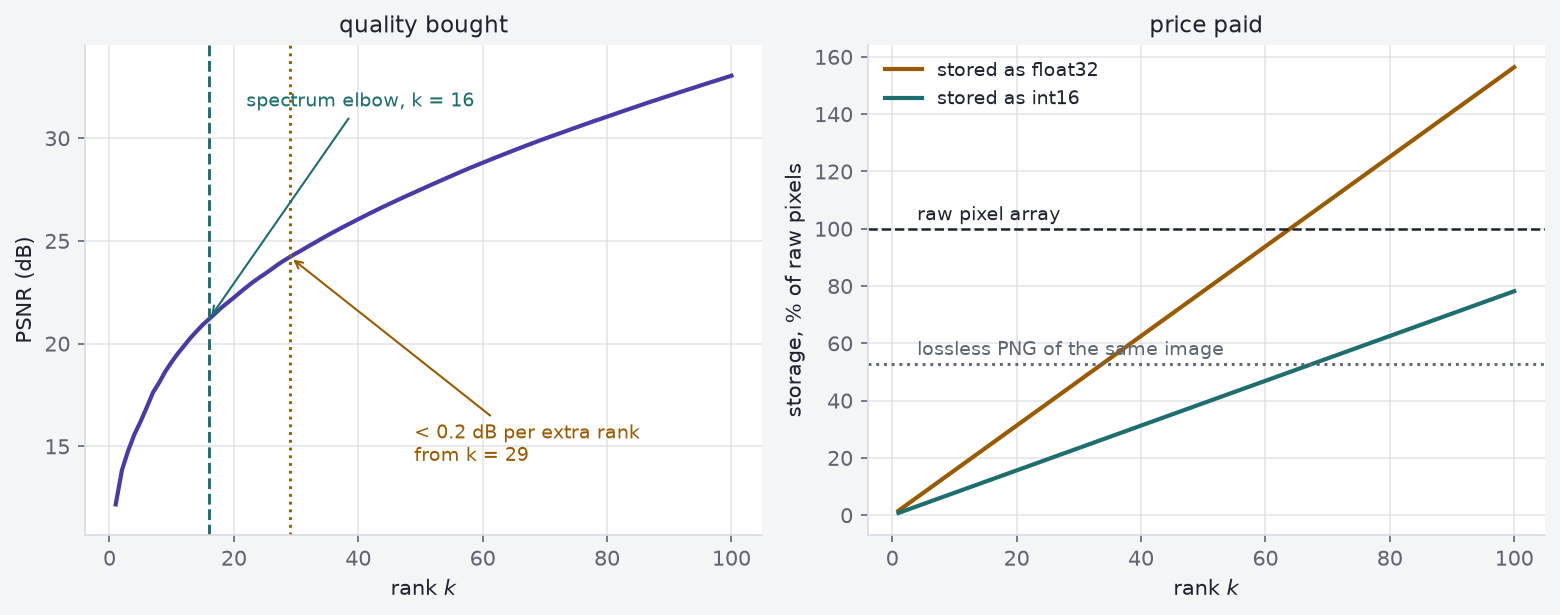
Figure 5: Left: reconstruction quality against rank, with the elbow of the singular value spectrum marked. Right: what the factors cost, as a fraction of the raw pixel array, under two storage choices. The float32 line crosses the raw-pixel baseline inside this range, so past that point the factorisation saves nothing.
k=   5  PSNR 16.21 dB   energy 91.492%   int16    3.9% of raw   float32    7.8%
k=  20  PSNR 22.24 dB   energy 97.830%   int16   15.6% of raw   float32   31.3%
k=  50  PSNR 27.50 dB   energy 99.349%   int16   39.1% of raw   float32   78.2%
k= 100  PSNR 33.04 dB   energy 99.818%   int16   78.2% of raw   float32  156.4%
The left panel shows where the returns stop: the spectrum bends at \(k = 16\) — the point furthest below a line drawn across the first 100 ranks, so it moves if you widen the window — and from \(k = 29\) onward each extra rank buys under a fifth of a decibel. The right panel is the part people skip. Stored naively as float32 the factors reach the size of the raw image at rank 64, and by rank 100 they take 156% of what you were trying to compress. Quantised to int16 — which the widget below does, at a quality cost too small to see — rank 50 costs 39% of raw for 27.5 dB.
Widget 2 — the rank dial100 triplets, 452 KB
The page ships the leading 100 singular triplets, not 100 images. Every rank you land on is rebuilt in the browser from those factors, which is the same trick that makes truncation useful in the first place: the generator is far smaller than what it generates.
5 Truncated SVD versus JPEG
Truncated SVD is the best rank-\(k\) approximation of a matrix. It is not the best image compressor, and the gap is not close.
SVD rank 20: 41,000 bytes, 22.24 dB
JPEG quality 5: 6,858 bytes, 25.92 dB
JPEG at its worst setting uses about a sixth of the bytes and still scores higher. It knows it is compressing an image: it works on local 8 × 8 blocks, discards high spatial frequencies the eye barely registers, and entropy-codes the rest. The SVD knows only that it has a matrix, and spends its budget on structure spanning the whole picture. Reach for truncation when the low-rank structure is itself what you care about, not when you want a smaller file.
5.1 The same dial, on ratings
Where low-rank structure is the point, the same truncation becomes a model. MovieLens 100k is 100,000 ratings on a 1–5 scale from real users of the MovieLens site, collected by the GroupLens group at the University of Minnesota, who ran the service partly to gather exactly this data for recommender research. As a matrix it is 943 users by 1,682 films and only about 6% filled — nearly every entry is a rating nobody gave. Predicting those wrong costs little each time and a lot in aggregate: a recommendation ignored, a film that never surfaces.
Truncation belongs here for a reason unrelated to storage. Taste is not 1,682-dimensional. If a few dozen latent factors explain most of what separates viewers, the ratings matrix is nearly low rank, and keeping the leading \(k\) layers keeps the signal while dropping one person’s mood on one evening. Where that boundary sits is empirical, so hold out 10% of the ratings and score reconstructions against them.
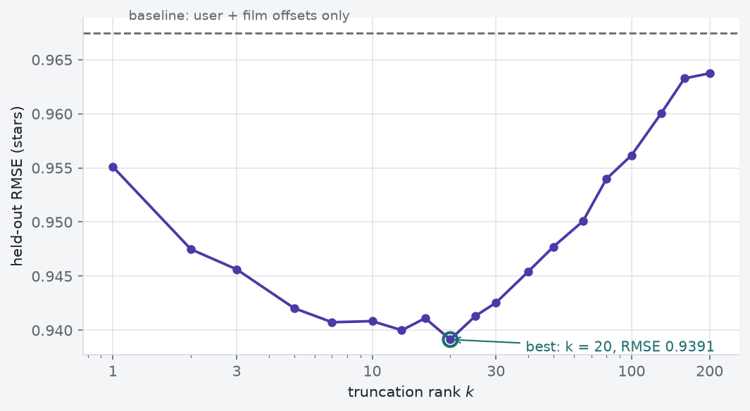
Figure 6: Held-out RMSE against truncation rank on MovieLens 100k, after removing per-user and per-film offsets. Too few ranks and the model has not learned taste; too many and it is memorising noise in the training ratings.
90,072 train / 9,928 test ratings, 5.7% of the matrix observed
The curve is a U. The photograph’s PSNR rose forever, because there the target was the matrix itself. Here the target is ratings the model has never seen, so past \(k = 20\) the extra layers fit the training ratings better and the held-out ratings worse. Rank has stopped being a compression setting and become a capacity knob.
5.2 The same dial, on ill-posed systems
Filip’s tiny singular values return here. Solving \(Ax = b\) through the SVD means computing \(x = \sum_i (u_i^\mathsf{T}b / \sigma_i) v_i\), and dividing by a \(\sigma_i\) of \(4 \times 10^{-6}\) amplifies whatever noise sits in that direction by a quarter of a million. Dropping the terms whose \(\sigma_i\) falls below a threshold is what np.linalg.pinv does by default — the same operation as dropping image layers, aimed at stability instead of storage. It trades a little bias for an answer that does not move when the data twitches, which is why it has a name of its own in the inverse problems literature: truncated SVD regularisation.
6 Avoid \(A^\mathsf{T}A\)
The derivation above reads like a recipe: form \(A^\mathsf{T}A\), diagonalise it, take square roots. Nobody does this, and Filip shows why in one line of output.
Squaring a matrix squares its condition number. If \(A\) has singular values \(\sigma_i\) then \(A^\mathsf{T}A\) has eigenvalues \(\sigma_i^2\), so \(\kappa(A^\mathsf{T}A) = \kappa(A)^2\): a matrix merely awkward at \(\kappa = 10^8\) becomes unsolvable at \(10^{16}\). The damage lands where it is least visible, on the small singular values — precisely where rank and regularisation decisions get made.
The largest singular value survives to full precision. The smallest does not survive at all: routed through \(A^\mathsf{T}A\) it comes back as exactly zero, so the matrix looks rank-deficient when it is not, while \(\sigma_{10}\) is too large by a factor of several hundred. Any rank decision taken from that column would be wrong. Working on \(A\) directly, np.linalg.svd puts \(\sigma_{11}\) at 4.071e-06 — small, but real.
LAPACK never forms \(A^\mathsf{T}A\). It squeezes \(A\) into bidiagonal form using Householder reflections — orthogonal, so they leave every length and therefore every singular value untouched — and only then diagonalises, iteratively, on the bidiagonal matrix.
flowchart LR
  A["<b>A</b><br/>m × n, dense"] -->|"Householder reflections<br/>left and right"| B["<b>B</b><br/>bidiagonal<br/>same singular values"]
  B -->|"implicit QR sweeps<br/>(Golub–Kahan)"| S["<b>Σ</b><br/>diagonal"]
  B -.->|"reflections<br/>accumulated"| UV["<b>U</b>, <b>V</b><br/>orthogonal factors"]
  S --> R["A = UΣVᵀ"]
  UV --> R
Figure 7: How a dense SVD is actually computed. Every arrow on the top row is an orthogonal transformation, so the singular values are identical at each stage; the condition number is never squared.
Which algorithm you want depends on how much of the decomposition you need.
method
cost
when to use it
full SVD — np.linalg.svd, LAPACK gesdd
\(O(mn \min(m, n))\)
you need every singular value, or the full \(U\) and \(V\), and the matrix fits in memory
eigendecomposition of \(A^\mathsf{T}A\)
\(O(mn^2 + n^3)\), at \(\kappa^2\)
effectively never — the cost saving is small and the accuracy loss is the one shown above
Lanczos — scipy.sparse.linalg.svds
\(O(k \cdot \mathrm{nnz}(A))\) per restart
\(k \ll n\) and the matrix is sparse, or reachable only as a matrix–vector product
\(k \ll n\), dense and large, and a small probabilistic error on the trailing singular values is acceptable
The bottom two rows are why a recommender on a hundred million ratings is tractable at all: nobody needs all 512 layers of the photograph, and nobody needs all 943 of MovieLens.
7 Three SVD questions
Three matrices have appeared so far — a photograph, a NIST design matrix, a table of ratings — and each asked something different of the same spectrum. Which leading layers are worth keeping. Which trailing directions will wreck a solver. How many layers the data can actually support. The catalogue of SVD applications is long, and almost none of it is a fourth question. It is these three, aimed at a matrix built from something other than pixels.
What changes between applications is what the rows and columns mean.
the matrix
rows × columns
what the spectrum gets read for
a grayscale photograph
pixels × pixels
how many layers before the eye stops noticing
a stack of face images
images × pixels
a face as a few dozen coordinates — “eigenfaces”
term–document counts
vocabulary × documents
topics, and words pulled together that never co-occur
a neural network’s weight matrix
outputs × inputs
parameters and inference time, traded against accuracy
centred measurements
samples × variables
the directions of most variance — PCA
a least-squares design matrix
observations × predictors
which coefficients the data cannot pin down
a rectangular or singular system
—
a pseudoinverse where no inverse exists
ratings
users × items
how many latent factors taste supports
a system’s impulse response
lags × lags, as a Hankel matrix
model order — which dynamic modes to keep
Two of those rows are worth spelling out, because in both cases the SVD is doing work under a name that hides it.
7.1 PCA is an SVD of the centred data, and the precision argument is why
Suppose you have a cloud of measurements — a few hundred samples, each with a few dozen numbers attached — and you want the directions along which the cloud is most spread out, because those are the directions carrying whatever the samples disagree about. That is principal component analysis, and the textbook recipe is to build the covariance matrix and diagonalise it: stack the samples as the rows of \(X\), subtract each column’s mean, and the sample covariance is \(X^\mathsf{T}X/(n-1)\).
But \(X^\mathsf{T}X\) is the matrix the whole decomposition was derived from. Its eigenvectors are exactly the right singular vectors \(v_i\) of \(X\), and its eigenvalues are exactly the \(\sigma_i^2\). So the principal components are the \(v_i\), the variance along the \(i\)-th is \(\sigma_i^2/(n-1)\), and the entire analysis is available from an SVD of the centred data with the covariance matrix never formed.
In exact arithmetic the two routes agree, so this looks like a matter of taste. The last section is what separates them: that was the same computation with different letters, and routed through the squared matrix the smallest singular value came back as exactly zero. As a PCA result that reads “this direction carries no variance at all” about a direction that carries some. Note which components take the damage. The ones that survive squaring are the ones you were going to keep anyway; the ones it destroys are the ones you were still deciding about.
Which does not make squaring forbidden — it makes it priced. sklearn’s PCA factors the centred matrix directly in most cases, but when the data is tall and skinny, at most a thousand variables and at least ten times as many samples, it forms the covariance matrix anyway, because a small square matrix is far faster to diagonalise than a tall one is to factor. That is speed bought with precision, on the bet that a thousand-column design is not Filip. The bet is usually right. What the spectrum gives you is the exchange rate: \(\kappa(A)^2\).
7.2 Truncating a term–document matrix invents topics nobody labelled
Words carry meaning through the company they keep, and a corpus records that company. Build a matrix with one row per vocabulary word and one column per document, each entry counting how often the word appears in it, usually weighted so that common words do not dominate. It comes out enormous and nearly empty — the same shape of problem as MovieLens, for the same reason: most words are absent from most documents.
Truncate it to a few hundred layers and something useful happens that nobody put in. Two words that never once appear in the same document can still end up with similar rows, if each keeps company with the same third set of words. The truncation has no choice: with only \(k\) layers to spend it cannot afford a separate direction for every word, so words that behave alike get folded onto shared directions. Those directions are the topics, and nobody labelled them. This is latent semantic analysis, from the late 1980s, and the rank knob behaves exactly as it did on ratings — too few layers and the topics are mush, too many and you are modelling one author’s word choice. The modern word embedding is the descendant: a different objective and a neural fitting procedure, still a low-rank factorisation of who-appears-near-whom.
Each of these keeps the leading layers because those are the interesting ones. None of them claims that what got discarded is nothing. There is one family where that stronger claim is close to literally true, and it is the one you can hear.
8 Hankel denoising
Sound arrives as one long vector, not a matrix — a few thousand samples per second and no second axis in sight. To use any of this you have to make a matrix out of it, and the standard construction is to slide a window along the signal and stack the windows as columns. Each column is the previous one shifted by a sample, so the matrix is constant along its anti-diagonals: a Hankel matrix, or in the time-series literature a trajectory matrix. It is the same object the impulse-response row of the table above refers to, which is why model reduction in control theory and denoising a recording are the same operation.
Building it looks wasteful — the thousand samples below become a matrix of a hundred and sixty thousand entries — but the redundancy is the point, because it forces the signal to declare its rank. A pure sinusoid obeys a two-term linear recurrence: any sample is a fixed combination of the two before it. So every window of it lies in a two-dimensional space, whatever the window length, and its trajectory matrix has rank exactly 2. A voiced sound is a stack of harmonics on one fundamental, so \(p\) harmonics give rank \(2p\) — a couple of dozen at most, in a matrix with hundreds of rows. White noise obeys no recurrence at all, so it spreads itself thinly across every direction there is.
That is the sharpest version of “keep the leading layers” in this post. On the photograph the cutoff was an elbow you had to eyeball; here the number of layers to keep is a count of harmonics, and the layers below it are noise by construction rather than by assumption.
The signal below is synthetic, and it has to be: subspace denoising can only be scored against a clean reference, and no recording of a real voice comes with one. It is five harmonics of a 120 Hz fundamental with amplitudes falling as \(1/k\), sampled at 8 kHz — a stand-in for a sustained vowel from a low-pitched speaker over a narrowband telephone line, where glottal pulses supply the harmonic stack and the vocal tract shapes how loud each one is. White Gaussian noise is added at 0 dB, meaning there is exactly as much noise energy as signal. What a decision here would affect is ordinary enough: this is the front of a hearing aid, a call centre’s line, or the audio a transcriber has to work from, and getting it wrong means either hiss the listener has to fight through or a voice with its edges smoothed off.
Code
import voice as vxt_v, clean = vx.vowel()noisy = vx.corrupt(clean, snr_db=0.0)sv_clean = np.linalg.svd(vx.trajectory(clean), compute_uv=False)sv_noisy = np.linalg.svd(vx.trajectory(noisy), compute_uv=False)print(f"signal: {clean.size} samples, {vx.FRAME}-sample windows "f"-> {vx.FRAME} x {clean.size - vx.FRAME +1} trajectory matrix")print(f"numerical rank of the clean trajectory matrix: "f"{int((sv_clean > sv_clean[0] *1e-10).sum())} (= 2 x {vx.N_HARM} harmonics)\n")print(f"{'i':>3s}{'clean':>10s}{'noisy':>10s}")for i in (0, 1, 8, 9, 10, 11, 20, 50):print(f"{i +1:3d}{sv_clean[i]:10.2f}{sv_noisy[i]:10.2f}")
signal: 1000 samples, 200-sample windows -> 200 x 801 trajectory matrix
numerical rank of the clean trajectory matrix: 10  (= 2 x 5 harmonics)

  i      clean      noisy
  1     234.09     221.91
  2     233.79     221.72
  9      46.82      56.62
 10      46.76      56.36
 11       0.00      44.82
 12       0.00      44.80
 21       0.00      40.38
 51       0.00      33.69
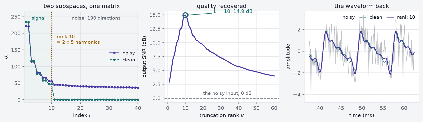
The clean matrix has numerical rank exactly 10, and its singular values arrive in near-equal pairs — one pair per harmonic, which is the rank-2 argument showing up in the arithmetic. Everything from \(\sigma_{11}\) down is zero to machine precision. Add the noise and those zeros lift to about 45, a floor that then decays slowly across the remaining 190 directions as the noise runs out of room. The strong harmonics barely notice — \(\sigma_1\) moves by 5% — while the weakest pair is close enough to the floor to be inflated by it, from 47 up to 57. That inflation is what 0 dB means here: the two subspaces are sorted into the same matrix with a step between them, but at this noise level the step is a step, not a chasm.
Keeping the top ten layers and folding the truncated matrix back into a signal — averaging along the anti-diagonals, since a truncated Hankel matrix is no longer quite Hankel — should therefore recover the vowel and leave the noise behind.
Figure 8: Left: singular values of the trajectory matrix, clean and noisy. The clean spectrum falls to zero after rank 10; the noisy one steps down at the same index onto a floor the noise puts there. Middle: recovered signal-to-noise ratio against truncation rank, peaking at exactly the rank the harmonics predict. Right: 25 ms of waveform, noisy against clean and against the rank-10 reconstruction.
input -0.00 dB -> rank 10: 14.92 dB (rank 5: 9.88, rank 40: 5.68)
The middle panel is the one to look at. The best rank is 10, which is \(2p\) for the \(p =\) 5 harmonics that went in — nothing in the code was told the answer, and the spectrum found it. It turns 0 dB into 14.9 dB, a factor of 31 in noise power, and the right panel shows what that means: the purple trace sits on the dashed clean one while the grey noise it came from wanders. Keep too few layers and harmonics go missing; keep too many and you are reconstructing noise along with the voice, and by rank 40 most of the gain is gone.
9 Synthetic vowel limits
The cliff in the left panel is that sharp because the synthetic vowel is exactly periodic and exactly stationary for the whole 125 ms. Real speech is neither. The fundamental drifts as the speaker’s pitch moves, the vocal tract reshapes continuously, and fricatives like /s/ and /f/ are not harmonic at all — they are noise, produced deliberately, and a rank cutoff cannot tell them from the noise you want gone. In practice the cliff softens into a slope and you are back to choosing a threshold, which is why real systems run this on frames of 20–30 ms at a time, or abandon the Hankel matrix for a spectrogram and truncate that instead. The mechanism survives; the free lunch does not.
9.1 The rest of a speech stack uses the same three questions
Denoising is the clearest case but not the only one, and the others are the familiar questions with audio-shaped matrices plugged in.
Speaker recognition builds a matrix of acoustic features — mel-frequency cepstral coefficients, a compact summary of a frame’s spectral shape — stacked over time, and reduces it to the few directions that separate one voice from another rather than one phoneme from another. The i-vector systems that ran speaker verification before neural embeddings took over pushed this furthest: a speaker became coordinates in a deliberately low-rank subspace of a much larger statistic, fitted by factor analysis rather than a bare SVD, but low-rank for exactly the reason MovieLens was. Older recognition pipelines did the same to their inputs, projecting stacked MFCCs down before handing them to a Gaussian mixture model, partly for speed and partly because the discarded directions were mostly redundant.
With more than one microphone the question becomes how many sources are in the room. Stack the channels and the rank of the resulting matrix counts the independent sources, up to the number of microphones — which is how a separation pipeline decides its model order before independent component analysis goes looking for the sources themselves, with the SVD usually doing the whitening step on the way. Voice activity detectors have been built on the same count run over short windows: a frame with someone talking in it is close to low rank, a frame of room tone is not. Dereverberation splits the same way, with the direct path concentrated in the leading directions and the reflections spread through the trailing ones.
10 Classical vs neural pipelines
For denoising, separation, recognition and verification, end-to-end neural models now beat these classical pipelines by margins that are not close, and have for about a decade. What is left for the subspace methods is real but narrower: lightweight baselines, deployments where a training set does not exist, and situations where you need to explain what the system did rather than only that it worked.
The exception runs the other way, and it is growing. The neural models that displaced these methods are themselves stacks of large weight matrices, and those matrices are often close to low rank — so the same truncation gets applied to the model instead of the audio, replacing an \(m \times n\) layer with two thin factors to shrink a speech model onto a phone. Low-rank adapters, the standard way to fine-tune a large model cheaply, are the same observation used for training instead of compression. Eckart–Young does not care whether the matrix holds pixels, ratings, a vowel or a weight.
11 Photograph summary
Rank 16: 97.2% Frobenius energy, 21.2 dB, 12.5% of raw bytes (int16 storage). Rank 50: 27.5 dB at 39% of raw.
Lossless PNG: 53% of raw. JPEG outperforms truncated SVD on bytes/quality for this image.