Maximum-Margin Classification from First Principles: SVMs as Convex Optimization

Why the widest street wins: geometry, quadratic programming, support vectors, and the soft-margin trade-off — every number below is solved, not asserted.

Machine Learning
Optimization
Mathematics
Author

Ravi Kalia

Published

July 23, 2026

Maximum-Margin Classification from First Principles

A support vector machine is often introduced as a bag of formulas: a hyperplane, a margin, a mysterious constant \(C\), and a dual problem that appears out of nowhere. This post rebuilds the linear SVM from the ground up around a single thread:

An SVM chooses a separating hyperplane by solving a convex optimization problem that maximizes geometric separation from the training data, while soft margins extend that idea to imperfectly separable data.

Everything is grounded in two tiny 2D datasets designed so you can check the geometry by eye. Every number reported — weights, intercepts, margins, support vectors, slack values — is computed by an actual convex solver (CVXPY) on the exact data plotted, and the notebook asserts that the solved values match the analytically derived ones before it will render. scikit-learn appears only at the end, as a cross-check.

Setup: imports, house palette, plotting helpers, and the toy dataset
import numpy as np
import cvxpy as cp
import matplotlib.pyplot as plt
from matplotlib.lines import Line2D
from IPython.display import Markdown

# palette (house style)
BLUE, ORANGE, INK = "#2a78d6", "#eb6834", "#0b0b0b"
MUTED, GRID, SURFACE = "#898781", "#e1e0d9", "#fcfcfb"

plt.rcParams.update({
    "figure.facecolor": SURFACE, "axes.facecolor": SURFACE,
    "savefig.facecolor": SURFACE,
    "axes.edgecolor": MUTED, "axes.labelcolor": INK,
    "xtick.color": MUTED, "ytick.color": MUTED, "text.color": INK,
    "axes.grid": True, "grid.color": GRID, "grid.linewidth": 0.8,
    "axes.spines.top": False, "axes.spines.right": False,
    "font.size": 11, "axes.titlesize": 12,
})

RNG_SEED = 42          # fixed seed for every random draw in this post
TOL = 1e-6             # numerical tolerance used for all constraint checks


def md_table(headers, rows):
    """Render a small Markdown table without extra dependencies."""
    head = "| " + " | ".join(headers) + " |"
    sep = "|" + "|".join(["---"] * len(headers)) + "|"
    body = ["| " + " | ".join(str(c) for c in r) + " |" for r in rows]
    return Markdown("\n".join([head, sep, *body]))


def scatter_classes(ax, X, y, s=70, sv_mask=None):
    """Class -1 as blue circles, class +1 as orange squares (shape backs up color)."""
    neg, pos = y < 0, y > 0
    ax.scatter(*X[neg].T, s=s, c=BLUE, marker="o", zorder=3,
               edgecolor=SURFACE, linewidth=1.2, label="class $-1$")
    ax.scatter(*X[pos].T, s=s, c=ORANGE, marker="s", zorder=3,
               edgecolor=SURFACE, linewidth=1.2, label="class $+1$")
    if sv_mask is not None and sv_mask.any():
        ax.scatter(*X[sv_mask].T, s=s * 3.4, facecolor="none",
                   edgecolor=INK, linewidth=1.6, zorder=4,
                   label="support vector")


def draw_hyperplane(ax, w, b, level=0.0, x1lim=(-1, 6), **kw):
    """Draw the line w@x + b = level over the given x1 range."""
    w = np.asarray(w, dtype=float)
    x1 = np.array(x1lim, dtype=float)
    if abs(w[1]) > 1e-12:
        ax.plot(x1, (level - b - w[0] * x1) / w[1], **kw)
    else:  # vertical line x1 = (level - b) / w1
        ax.axvline((level - b) / w[0], **kw)


def draw_svm(ax, w, b, x1lim=(-1, 6)):
    """Decision boundary plus the two margin lines w@x + b = ±1."""
    draw_hyperplane(ax, w, b, 0.0, x1lim, color=INK, lw=2.0,
                    label=r"boundary $w^\top x + b = 0$")
    for lv in (-1.0, 1.0):
        draw_hyperplane(ax, w, b, lv, x1lim, color=MUTED, lw=1.4, ls="--",
                        label=r"margin $w^\top x + b = \pm 1$" if lv > 0 else None)


# ---- Dataset A: linearly separable, chosen for clean numbers -----------------
X_A = np.array([
    [1.0, 1.0], [0.0, 1.5], [1.5, 0.0], [0.3, 0.4], [1.2, 0.2],   # class -1
    [3.0, 3.0], [2.8, 3.4], [3.5, 4.0], [4.0, 2.5], [4.5, 3.2],   # class +1
])
y_A = np.array([-1, -1, -1, -1, -1, +1, +1, +1, +1, +1])
n_A = len(y_A)

1 The geometric classification problem

We start with Dataset A: ten points in the plane, five per class, with labels \(y_i \in \{-1, +1\}\). The coordinates are deliberately simple — the two classes sit in opposite corners with a visible corridor between them.

A linear classifier is a function

\[ f(x) = w^\top x + b, \]

where \(w \in \mathbb{R}^2\) is a normal vector perpendicular to the decision boundary and \(b \in \mathbb{R}\) is an intercept. We predict class \(+1\) when \(f(x) > 0\) and class \(-1\) when \(f(x) < 0\); the decision boundary is the line \(\{x : w^\top x + b = 0\}\).

A hyperplane separates the training data when every point lands on its own class’s side, which is captured in one inequality per point:

\[ y_i \left( w^\top x_i + b \right) > 0, \qquad i = 1, \ldots, n. \]

Multiplying by the label is a compact trick: for a \(+1\) point it requires \(f(x_i) > 0\), and for a \(-1\) point it flips the inequality to require \(f(x_i) < 0\). One formula, both cases.

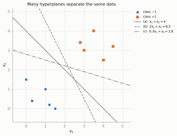
Here is the immediate problem: separability does not pick a classifier. The cell below defines three hand-chosen candidate lines, verifies numerically that each one separates Dataset A perfectly (minimum of \(y_i f(x_i)\) over the data is strictly positive), and plots them. All three achieve 100% training accuracy. Which should we prefer?

Verify and plot three separating lines
candidates = {
    "(a)  $x_1 + x_2 = 4$":            (np.array([1.0, 1.0]),  -4.0),
    "(b)  $2x_1 + x_2 = 6.5$":         (np.array([2.0, 1.0]),  -6.5),
    "(c)  $0.3x_1 + x_2 = 2.8$":       (np.array([0.3, 1.0]),  -2.8),
}
for name, (w_c, b_c) in candidates.items():
    worst = np.min(y_A * (X_A @ w_c + b_c))
    assert worst > 0, f"candidate {name} does not separate the data"

fig, ax = plt.subplots(figsize=(7.5, 5.6))
scatter_classes(ax, X_A, y_A)
for (name, (w_c, b_c)), ls in zip(candidates.items(), ["-", "--", "-."]):
    draw_hyperplane(ax, w_c, b_c, 0.0, (-1, 6), color=MUTED, lw=1.8, ls=ls,
                    label=name)
ax.set_xlim(-0.7, 5.4); ax.set_ylim(-0.7, 5.2); ax.set_aspect("equal")
ax.set_xlabel("$x_1$"); ax.set_ylabel("$x_2$")
ax.legend(frameon=False, loc="upper left", bbox_to_anchor=(1.01, 1.0),
          fontsize=9)
ax.set_title("Many hyperplanes separate the same data")
plt.tight_layout()
plt.show()
Figure 1: Three different lines, each verified to classify all ten training points correctly. Training accuracy alone cannot choose between them — line (c) skims dangerously close to the blue class, yet separates the data just as ‘perfectly’ as the others.

All three lines are feasible, but they are not equally trustworthy. Line (c) passes so close to the blue class that a tiny perturbation of one point would flip its predicted label. Intuitively, we want the line with the most clearance — the widest empty corridor between it and the nearest data. The rest of the post makes that intuition exact.

2 Margin from first principles

2.1 Distance from a point to a hyperplane

The tool we need is the perpendicular distance from a point \(x_i\) to the line \(\{x : w^\top x + b = 0\}\). Since \(w\) is normal to the line, projecting onto the unit normal \(w / \lVert w \rVert\) gives

\[ \operatorname{dist}(x_i) \;=\; \frac{\left| w^\top x_i + b \right|}{\lVert w \rVert}. \]

The numerator \(|f(x_i)|\) is called the functional margin — it depends on how \((w, b)\) is scaled. Dividing by \(\lVert w \rVert\) converts it into the scale-free geometric margin, an actual distance in the plane.

Define the margin of a separating hyperplane as its distance to the closest training point:

\[ \gamma(w, b) \;=\; \min_i \frac{y_i \left( w^\top x_i + b \right)}{\lVert w \rVert}. \]

Now we can score the three candidate lines from Figure 1 instead of merely checking feasibility:

Geometric margin of each candidate line
rows = []
for name, (w_c, b_c) in candidates.items():
    d = y_A * (X_A @ w_c + b_c) / np.linalg.norm(w_c)
    rows.append([name, f"{d.min():.3f}",
                 f"({X_A[d.argmin()][0]:g}, {X_A[d.argmin()][1]:g})"])
md_table(["candidate line", "geometric margin $\\gamma$ (distance)",
          "closest training point"], rows)
candidate line geometric margin \(\gamma\) (distance) closest training point
(a) \(x_1 + x_2 = 4\) 1.414 (1, 1)
(b) \(2x_1 + x_2 = 6.5\) 1.118 (3, 3)
(c) \(0.3x_1 + x_2 = 2.8\) 0.862 (4, 2.5)

Line (a) keeps every point at least \(\sqrt{2} \approx 1.414\) units away; line (c) manages barely \(0.86\). “Maximize the margin” now has a precise meaning: among all separating \((w, b)\), find the one with the largest \(\gamma\).

2.2 The scaling ambiguity and the canonical form

There is a wrinkle. The pairs \((w, b)\) and \((cw, cb)\) describe the same line for any \(c > 0\) — every functional margin gets multiplied by \(c\), but the geometric margin \(\gamma\) is unchanged because the \(\lVert w \rVert\) in the denominator absorbs it. So the parametrization is redundant, and “maximize \(\gamma\)” as written is an awkward, non-smooth objective over a redundant space.

The classical fix is to spend the redundancy: rescale \((w, b)\) so that the closest points have functional margin exactly 1. That is, impose the canonical constraints

\[ y_i \left( w^\top x_i + b \right) \ge 1, \qquad i = 1, \ldots, n, \]

with equality holding for the nearest point(s). Under this convention the nearest points sit at geometric distance

\[ \frac{y_i \left( w^\top x_i + b \right)}{\lVert w \rVert} = \frac{1}{\lVert w \rVert} \]

from the boundary. Two distinct quantities follow, and it pays to keep them straight:

  • the one-sided geometric margin — boundary to the nearest point on either side: \(1 / \lVert w \rVert\);
  • the full margin width — the whole empty band from the margin line \(w^\top x + b = -1\) across to \(w^\top x + b = +1\): \(2 / \lVert w \rVert\).

When people say “the margin” they usually mean the band width \(2/\lVert w \rVert\), but plots of “the margin lines” show the two one-sided boundaries. Both appear in the figures below.

3 The hard-margin primal problem

Under canonical scaling, maximizing the margin \(1 / \lVert w \rVert\) is the same as minimizing \(\lVert w \rVert\), and minimizing \(\lVert w \rVert\) is the same as minimizing the smooth, differentiable quantity \(\tfrac12 \lVert w \rVert^2\) (the \(\tfrac12\) just tidies derivatives). That gives the hard-margin SVM primal:

\[ \begin{aligned} \min_{w, b} \quad & \tfrac{1}{2} \lVert w \rVert^2 \\ \text{subject to} \quad & y_i \left( w^\top x_i + b \right) \ge 1, \qquad i = 1, \ldots, n. \end{aligned} \]

In words: among all hyperplanes that classify every training point correctly with functional margin at least 1, pick the one whose normal vector is shortest — equivalently, whose geometric margin \(1/\lVert w \rVert\) is widest. The constraints do the separating; the objective does the margin-maximizing.

3.1 Solving it with CVXPY

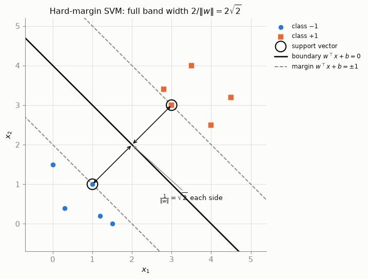
Dataset A was constructed so the answer is knowable in advance: the closest pair of points across the class gap is \((1,1)\) and \((3,3)\), so the optimal boundary should be their perpendicular bisector \(x_1 + x_2 = 4\) — candidate (a) from earlier — with \(w^\star = (0.5,\, 0.5)\), \(b^\star = -2\), and margin width \(2/\lVert w^\star \rVert = 2\sqrt{2}\). The cell below solves the QP and asserts that the solver agrees, so this post cannot render with numbers that contradict its own prose.

Hard-margin QP in CVXPY, with assertions against the analytic solution
w = cp.Variable(2)
b = cp.Variable()
margin_cons = [cp.multiply(y_A, X_A @ w + b) >= 1]
hard = cp.Problem(cp.Minimize(0.5 * cp.sum_squares(w)), margin_cons)
hard.solve(solver=cp.CLARABEL)

w_hard, b_hard = w.value, b.value
alpha_hard = margin_cons[0].dual_value        # Lagrange multipliers (used later)
func_margins = y_A * (X_A @ w_hard + b_hard)
sv_mask_hard = np.isclose(func_margins, 1.0, atol=1e-4)
width_hard = 2 / np.linalg.norm(w_hard)

assert hard.status == "optimal"
assert np.allclose(w_hard, [0.5, 0.5], atol=1e-5), w_hard
assert abs(b_hard - (-2.0)) < 1e-5, b_hard
assert func_margins.min() >= 1 - TOL           # all constraints satisfied
assert sv_mask_hard.sum() == 2                 # exactly (1,1) and (3,3)

print(f"solver status   : {hard.status}")
print(f"w* = ({w_hard[0]:.6f}, {w_hard[1]:.6f}),  b* = {b_hard:.6f}")
print(f"decision boundary: {w_hard[0]:.3f}·x1 + {w_hard[1]:.3f}·x2 "
      f"+ {b_hard:.3f} = 0   (i.e. x1 + x2 = 4)")
print(f"one-sided margin : 1/||w|| = {1/np.linalg.norm(w_hard):.6f}  (= √2)")
print(f"full margin width: 2/||w|| = {width_hard:.6f}  (= 2√2)")
print(f"support vectors  : {[tuple(p) for p in X_A[sv_mask_hard]]}")
print(f"min_i y_i(w·x_i+b) = {func_margins.min():.8f}  (≥ 1 − {TOL:g} ✓)")
solver status   : optimal
w* = (0.500000, 0.500000),  b* = -2.000000
decision boundary: 0.500·x1 + 0.500·x2 + -2.000 = 0   (i.e. x1 + x2 = 4)
one-sided margin : 1/||w|| = 1.414214  (= √2)
full margin width: 2/||w|| = 2.828427  (= 2√2)
support vectors  : [(np.float64(1.0), np.float64(1.0)), (np.float64(3.0), np.float64(3.0))]
min_i y_i(w·x_i+b) = 1.00000000  (≥ 1 − 1e-06 ✓)

The solver recovers the analytic solution to six decimal places. The per-point constraint values make the geometry concrete — a functional margin of exactly \(1\) marks a support vector, anything larger means the point sits strictly outside the margin band:

Per-point constraint check
rows = []
for i in range(n_A):
    rows.append([
        f"({X_A[i,0]:g}, {X_A[i,1]:g})", f"{y_A[i]:+d}",
        f"{func_margins[i]:.4f}",
        f"{func_margins[i]/np.linalg.norm(w_hard):.4f}",
        "**support vector**" if sv_mask_hard[i] else "interior",
    ])
md_table(["$x_i$", "$y_i$", "$y_i(w^\\top x_i + b)$",
          "distance to boundary", "role"], rows)
\(x_i\) \(y_i\) \(y_i(w^\top x_i + b)\) distance to boundary role
(1, 1) -1 1.0000 1.4142 support vector
(0, 1.5) -1 1.2500 1.7678 interior
(1.5, 0) -1 1.2500 1.7678 interior
(0.3, 0.4) -1 1.6500 2.3335 interior
(1.2, 0.2) -1 1.3000 1.8385 interior
(3, 3) +1 1.0000 1.4142 support vector
(2.8, 3.4) +1 1.1000 1.5556 interior
(3.5, 4) +1 1.7500 2.4749 interior
(4, 2.5) +1 1.2500 1.7678 interior
(4.5, 3.2) +1 1.8500 2.6163 interior

Only the two support vectors touch the constraint boundary \(y_i f(x_i) = 1\); the other eight constraints are slack (inactive). Delete any non-support point and re-solve — the answer would not move. The two support vectors are the solution’s memory of the data.

Plot the hard-margin solution
fig, ax = plt.subplots(figsize=(7.5, 5.8))
scatter_classes(ax, X_A, y_A, sv_mask=sv_mask_hard)
draw_svm(ax, w_hard, b_hard)

# perpendicular distance arrows from each support vector to the boundary
u = w_hard / np.linalg.norm(w_hard)          # unit normal
for sv, sign in zip(X_A[sv_mask_hard], (-1, +1)):
    foot = sv - (w_hard @ sv + b_hard) / np.linalg.norm(w_hard) * u
    ax.annotate("", xy=foot, xytext=sv,
                arrowprops=dict(arrowstyle="<->", color=INK, lw=1.2))
ax.annotate(r"$\frac{1}{\Vert w\Vert}=\sqrt{2}$ each side",
            xy=(2.0, 2.0), xytext=(2.7, 0.6), fontsize=10,
            arrowprops=dict(arrowstyle="->", color=MUTED))
ax.set_xlim(-0.7, 5.4); ax.set_ylim(-0.7, 5.2); ax.set_aspect("equal")
ax.set_xlabel("$x_1$"); ax.set_ylabel("$x_2$")
ax.legend(frameon=False, loc="upper left", bbox_to_anchor=(1.01, 1.0),
          fontsize=9)
ax.set_title(r"Hard-margin SVM: full band width $2/\Vert w\Vert = 2\sqrt{2}$")
plt.tight_layout()
plt.show()
Figure 2: The maximum-margin solution for Dataset A: boundary \(x_1+x_2=4\) (solid), margin lines \(w^\top x + b = \pm 1\) (dashed), support vectors ringed in black. Each support vector sits exactly \(1/\lVert w\rVert = \sqrt{2}\) from the boundary; the full band is \(2\sqrt{2} \approx 2.83\) wide.

4 Why this is convex optimization

The hard-margin problem is a convex quadratic program (QP), and each ingredient is worth naming:

  • The objective is convex. \(\tfrac12\lVert w \rVert^2 = \tfrac12(w_1^2 + w_2^2)\) is a paraboloid — its Hessian is the identity, which is positive definite, so it is strictly convex in \(w\). (Note \(b\) does not appear in the objective at all; as a function of the joint variable \((w, b)\) the objective is convex but not strictly convex. This detail matters for uniqueness, below.)
  • Each constraint is a half-space in parameter space. For a fixed data point \((x_i, y_i)\), the set \(\{(w, b) : y_i(w^\top x_i + b) \ge 1\}\) is defined by a single linear inequality in the unknowns \((w, b)\) — a half-space in \(\mathbb{R}^3\). This is the perspective flip that makes SVMs tractable: each data point becomes a linear constraint on the parameters.
  • The feasible region is convex. An intersection of half-spaces (a polyhedron) is always convex.

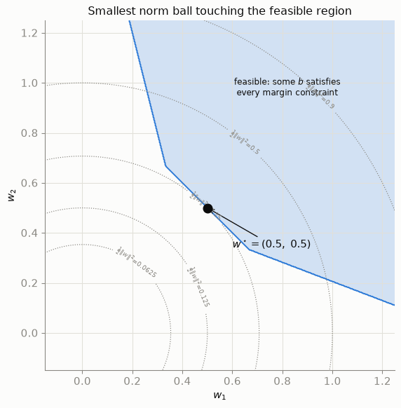
Minimizing a convex function over a convex set is exactly the definition of a convex optimization problem. To draw the feasible set we need one small maneuver: the full feasible region lives in \((w_1, w_2, b)\)-space, and slicing it at the optimal \(b^\star\) is useless — at the optimum the two support-vector constraints are tight, so that slice degenerates to a line segment with no area to shade. Instead we eliminate \(b\): a given \(w\) admits some feasible intercept exactly when \(\max_{i \in +} (1 - w^\top x_i) \le \min_{j \in -} (-1 - w^\top x_j)\), i.e. when

\[ w^\top (x_i - x_j) \ge 2 \qquad \text{for every cross-class pair } (i \in +,\ j \in -), \]

which is again an intersection of half-planes — now purely in \((w_1, w_2)\), so we can plot it, along with the circular level sets of \(\tfrac12\lVert w\rVert^2\) and the optimum where the smallest circle touches the region.

Feasible region in (w1, w2) after eliminating b
g = np.linspace(-0.15, 1.25, 500)
W1, W2 = np.meshgrid(g, g)
feasible = np.ones_like(W1, dtype=bool)
for xp in X_A[y_A > 0]:
    for xn in X_A[y_A < 0]:
        d = xp - xn
        feasible &= (W1 * d[0] + W2 * d[1]) >= 2

fig, ax = plt.subplots(figsize=(6.8, 6.2))
ax.contourf(W1, W2, feasible.astype(float), levels=[0.5, 1.5],
            colors=["#2a78d633"])
ax.contour(W1, W2, feasible.astype(float), levels=[0.5],
           colors=[BLUE], linewidths=1.4)
R = np.sqrt(W1**2 + W2**2)
cs = ax.contour(W1, W2, 0.5 * R**2, levels=[0.0625, 0.125, 0.25, 0.5, 0.9],
                colors=[MUTED], linewidths=0.9, linestyles=":")
ax.clabel(cs, fmt=lambda v: rf"$\frac{{1}}{{2}}\|w\|^2$={v:g}", fontsize=7)
ax.scatter([w_hard[0]], [w_hard[1]], s=90, c=INK, zorder=5)
ax.annotate(r"$w^\star = (0.5,\ 0.5)$", xy=w_hard, xytext=(0.60, 0.34),
            fontsize=11, arrowprops=dict(arrowstyle="->", color=INK))
ax.annotate("feasible: some $b$ satisfies\nevery margin constraint",
            xy=(0.82, 0.95), fontsize=9, color=INK, ha="center")
ax.set_xlabel("$w_1$"); ax.set_ylabel("$w_2$"); ax.set_aspect("equal")
ax.set_title("Smallest norm ball touching the feasible region")
plt.tight_layout()
plt.show()
Figure 3: The QP in parameter space with the intercept eliminated: each cross-class pair of training points imposes the half-plane \(w^\top(x_i - x_j) \ge 2\) on \((w_1, w_2)\); their intersection is the shaded feasible region. The objective’s circular level sets shrink toward the origin, and \(w^\star = (0.5, 0.5)\) is the point of the feasible region closest to the origin — its active edge is generated by the support-vector pair \((3,3)\) and \((1,1)\).

4.1 What convexity buys you

  • Every local optimum is a global optimum. A convex landscape has no false bottoms: if no feasible descent direction exists at a point, no better feasible point exists anywhere.
  • Solvers can target the global optimum, not just a stationary point, and can certify optimality via duality (a matching lower bound). CLARABEL, the interior-point solver used above, reports optimal — a certificate, not a hope.
  • There are no distinct “bad local minima” to escape, so no restarts, annealing, or initialization tricks are needed.

4.2 What convexity does not buy you

  • Feasibility. If no hyperplane separates the data, the constraint set is empty and the hard-margin problem has no solution at all. (We will hit this in Section 7 — the solver honestly reports infeasible.)
  • Uniqueness of the optimizer. Convexity guarantees the set of optima is convex, not that it is a single point. Extra conditions are needed.
  • Numerical immunity. Finite-precision solvers return answers to a tolerance (note the 1e-6 and 1e-4 tolerances used throughout this post); badly conditioned or nearly degenerate problems can stress them.

The uniqueness question deserves precision, because the objective is strictly convex in \(w\) but \(b\) never appears in it:

  • \(w^\star\) is always unique (when the problem is feasible): if two optima had different \(w\)’s, their midpoint would be feasible (convexity) with strictly smaller \(\tfrac12\lVert w\rVert^2\) (strict convexity) — contradiction.
  • \(b^\star\) requires an argument. Given \(w^\star\), the constraints pin \(b\) into an interval \([\,b_{\text{lo}},\, b_{\text{hi}}\,]\) where \(b_{\text{lo}}\) comes from the \(+1\) class and \(b_{\text{hi}}\) from the \(-1\) class. For a separable two-class problem this interval collapses to a point: if it had positive length, an interior \(b\) would leave every constraint slack, and \((w, b)\) could be scaled down to a feasible point with smaller norm — contradicting optimality of \(w^\star\). So the standard two-class hard-margin solution \((w^\star, b^\star)\) — and hence the geometric boundary — is unique.
  • Degenerate formulations can break this, as the next section shows with actual solves: \(b\) (and even the existence of a boundary) can fail to be pinned down.

5 Making uniqueness concrete

5.1 The generic case: Dataset A’s solution is unique

Following the argument above, we compute the interval of intercepts compatible with \(w^\star\) and check it collapses; and we re-solve the same QP with two different solver algorithms (interior-point CLARABEL and first-order OSQP) to see them agree:

b-interval collapse + independent solvers agree
b_lo = np.max(1 - X_A[y_A > 0] @ w_hard)      # +1 class: b ≥ 1 − w·x
b_hi = np.min(-1 - X_A[y_A < 0] @ w_hard)     # −1 class: b ≤ −1 − w·x
print(f"b interval given w*: [{b_lo:.6f}, {b_hi:.6f}]  →  width "
      f"{b_hi - b_lo:.2e} (collapses to the point b* = −2)")

hard.solve(solver=cp.OSQP)
print(f"OSQP     : w = ({w.value[0]:.6f}, {w.value[1]:.6f}), b = {b.value:.6f}")
print(f"CLARABEL : w = ({w_hard[0]:.6f}, {w_hard[1]:.6f}), b = {b_hard:.6f}")
assert np.allclose(w.value, w_hard, atol=1e-3) and abs(b.value - b_hard) < 1e-3
hard.solve(solver=cp.CLARABEL)   # restore the reference solution
b interval given w*: [-2.000000, -2.000000]  →  width 3.11e-10 (collapses to the point b* = −2)
OSQP     : w = (0.500000, 0.500000), b = -2.000000
CLARABEL : w = (0.500000, 0.500000), b = -2.000000
np.float64(0.25000000007783907)

Two very different algorithms land on the same \((w^\star, b^\star)\) — as they must, since the optimum is a single point.

5.2 A genuinely degenerate case: one class only

Feed the hard-margin QP only the five \(+1\) points and it is still a perfectly valid convex program — but the constraints \(w^\top x_i + b \ge 1\) can be satisfied with \(w = 0,\ b \ge 1\), which achieves the unbeatable objective value \(0\). The optimal set is the entire ray \(\{(0, b) : b \ge 1\}\):

  • \(w^\star = 0\) is unique (strict convexity in \(w\) still applies),
  • \(b^\star\) is wildly non-unique — any \(b \ge 1\) is optimal,
  • and with \(w^\star = 0\) there is no decision boundary at all: the “hyperplane” \(0^\top x + b = 0\) is not a hyperplane.
One-class degenerate solve with two solvers
w1c, b1c = cp.Variable(2), cp.Variable()
one_class = cp.Problem(cp.Minimize(0.5 * cp.sum_squares(w1c)),
                       [X_A[y_A > 0] @ w1c + b1c >= 1])
for solver in (cp.CLARABEL, cp.SCS):
    one_class.solve(solver=solver)
    print(f"{solver:<9}: status={one_class.status},  ||w|| = "
          f"{np.linalg.norm(w1c.value):.2e},  b = {b1c.value:.4f}")
    assert np.linalg.norm(w1c.value) < 1e-3   # w* = 0 in both cases
CLARABEL : status=optimal,  ||w|| = 5.25e-10,  b = 3.0166
SCS      : status=optimal,  ||w|| = 4.87e-12,  b = 1.0000

Both solvers agree that \(w^\star = 0\), but each returns whatever intercept its algorithm happened to stop at — both answers are equally “optimal” because the constraints never pin \(b\) down. This is non-uniqueness of a degenerate formulation, honestly labeled: it is not evidence that ordinary two-class hard-margin SVMs have multiple solutions (they do not, as shown above). A cleaner and more practically relevant failure of uniqueness — an interval of equally optimal intercepts for a genuine two-class problem — appears once soft margins enter, in Section 7.3.

A caution about symmetry: it is tempting to think a symmetric dataset must admit multiple maximum-margin hyperplanes. Usually the opposite is true — by uniqueness, the one optimal hyperplane must itself be invariant under any symmetry of the data (swap the classes of Dataset A’s support vectors across the corridor and the boundary \(x_1 + x_2 = 4\) maps to itself). Symmetry constrains the unique solution; it does not multiply it.

6 Lagrangian and dual intuition

Where do “support vectors” get their name and their power? From duality. Attach a multiplier \(\alpha_i \ge 0\) to each constraint and form the Lagrangian

\[ \mathcal{L}(w, b, \alpha) = \tfrac12 \lVert w \rVert^2 - \sum_{i} \alpha_i \left[ y_i \left( w^\top x_i + b \right) - 1 \right]. \]

Setting the derivatives with respect to the primal variables to zero gives the stationarity conditions

\[ \frac{\partial \mathcal{L}}{\partial w} = 0 \;\;\Rightarrow\;\; w = \sum_i \alpha_i y_i x_i, \qquad\qquad \frac{\partial \mathcal{L}}{\partial b} = 0 \;\;\Rightarrow\;\; \sum_i \alpha_i y_i = 0. \]

Two consequences, both checkable on our solved problem:

  1. The optimal \(w\) is a weighted combination of data points. Complementary slackness (\(\alpha_i \cdot [\text{slack of constraint } i] = 0\)) forces \(\alpha_i = 0\) for every point whose constraint is inactive — every point strictly outside the margin. Only points on the margin can carry weight. That is why they support the hyperplane.
  2. The weights balance across classes (\(\sum_i \alpha_i y_i = 0\)): the positive-class pull equals the negative-class pull, which is why the boundary settles in equilibrium between the classes.

CVXPY hands us the optimal multipliers as the constraint’s dual_value. For Dataset A the analytic prediction is \(\alpha = 0.25\) for each support vector (solve \(\alpha \cdot \big[(3,3)-(1,1)\big] = w^\star\) with balanced weights) and \(0\) elsewhere:

Dual variables: support vectors carry all the weight
rows = [[f"({X_A[i,0]:g}, {X_A[i,1]:g})", f"{y_A[i]:+d}",
         f"{alpha_hard[i]:.6f}",
         f"{alpha_hard[i] * (func_margins[i] - 1):.1e}"]
        for i in range(n_A)]
display(md_table(["$x_i$", "$y_i$", "$\\alpha_i$",
                  "$\\alpha_i\\,[y_i f(x_i) - 1]$ (compl. slack)"], rows))

w_from_alpha = (alpha_hard * y_A) @ X_A
dual_val = alpha_hard.sum() - 0.5 * np.linalg.norm(w_from_alpha) ** 2
print(f"stationarity  ||w* − Σαᵢyᵢxᵢ||  = "
      f"{np.linalg.norm(w_hard - w_from_alpha):.2e}")
print(f"balance        Σαᵢyᵢ           = {(alpha_hard * y_A).sum():+.2e}")
print(f"strong duality: dual objective  = {dual_val:.6f} "
      f"vs primal ½||w*||² = {0.5*np.linalg.norm(w_hard)**2:.6f}")
assert np.allclose(alpha_hard[sv_mask_hard], 0.25, atol=1e-4)
assert np.all(alpha_hard[~sv_mask_hard] < 1e-6)
\(x_i\) \(y_i\) \(\alpha_i\) \(\alpha_i\,[y_i f(x_i) - 1]\) (compl. slack)
(1, 1) -1 0.250000 4.4e-11
(0, 1.5) -1 0.000000 2.8e-11
(1.5, 0) -1 0.000000 4.4e-11
(0.3, 0.4) -1 0.000000 4.2e-11
(1.2, 0.2) -1 0.000000 4.0e-11
(3, 3) +1 0.250000 3.4e-11
(2.8, 3.4) +1 0.000000 5.7e-11
(3.5, 4) +1 0.000000 4.0e-11
(4, 2.5) +1 0.000000 3.4e-11
(4.5, 3.2) +1 0.000000 3.8e-11
stationarity  ||w* − Σαᵢyᵢxᵢ||  = 2.33e-10
balance        Σαᵢyᵢ           = -6.50e-11
strong duality: dual objective  = 0.250000 vs primal ½||w*||² = 0.250000

Eight of ten points have \(\alpha_i = 0\): as far as the optimization is concerned, they might as well not exist. Substituting the stationarity conditions back into \(\mathcal{L}\) yields the dual problem

\[ \max_{\alpha \ge 0,\ \sum_i \alpha_i y_i = 0} \;\; \sum_i \alpha_i - \tfrac12 \sum_{i,j} \alpha_i \alpha_j y_i y_j \, x_i^\top x_j, \]

whose value (\(0.25\), printed above) matches the primal optimum exactly — strong duality. Notice the data enters the dual only through dot products \(x_i^\top x_j\). That single observation is the doorway to kernel methods — replace the dot product with a kernel function and everything above survives — but linear geometry is enough for this post, so we leave that door ajar.

7 Soft margins for non-separable data

Real data rarely offers a clean corridor. Dataset B below draws two overlapping Gaussian blobs (fixed seed) and adds one blue outlier deep inside orange territory. First, an honest check that the hard-margin machinery genuinely breaks here — the constraint set is empty and the solver says so:

Dataset B + hard margin is infeasible on it
rng = np.random.default_rng(RNG_SEED)
X_neg = rng.normal(loc=[1.4, 1.6], scale=0.75, size=(20, 2))
X_pos = rng.normal(loc=[3.3, 3.1], scale=0.75, size=(20, 2))
outlier = np.array([[4.3, 3.7]])                       # labeled −1, sits among +1
X_B = np.vstack([X_neg, outlier, X_pos])
y_B = np.array([-1] * 21 + [+1] * 20)
n_B = len(y_B)

wi, bi = cp.Variable(2), cp.Variable()
infeas = cp.Problem(cp.Minimize(0.5 * cp.sum_squares(wi)),
                    [cp.multiply(y_B, X_B @ wi + bi) >= 1])
infeas.solve(solver=cp.CLARABEL)
print(f"hard margin on Dataset B: status = {infeas.status}")
assert infeas.status == "infeasible"
hard margin on Dataset B: status = infeasible

7.1 Slack variables

The soft-margin SVM keeps the same objective and constraints but lets each point buy its way out of its constraint with a slack variable \(\xi_i \ge 0\), at a price \(C\) per unit:

\[ \begin{aligned} \min_{w, b, \xi} \quad & \tfrac12 \lVert w \rVert^2 + C \sum_i \xi_i \\ \text{subject to} \quad & y_i \left( w^\top x_i + b \right) \ge 1 - \xi_i, \\ & \xi_i \ge 0, \qquad i = 1, \ldots, n. \end{aligned} \]

This is still a convex QP — the objective gains a linear term, the constraints stay linear — so everything from the convexity section carries over. At the optimum, \(\xi_i = \max\!\big(0,\, 1 - y_i f(x_i)\big)\), and its value tells you exactly where the point ended up:

  • \(\xi_i = 0\): correctly classified, on or outside the margin — the constraint needed no help;
  • \(0 < \xi_i \le 1\): correctly classified but inside the margin band;
  • \(\xi_i > 1\): misclassified (\(y_i f(x_i) < 0\); at \(\xi_i = 1\) the point sits exactly on the boundary).

\(C\) is the exchange rate between the two goals: margin width versus violation. We solve for a small, medium, and large \(C\):

Solve the soft-margin QP for three values of C
def solve_soft(X, y, C, solver=cp.CLARABEL):
    n = len(y)
    w_, b_, xi_ = cp.Variable(2), cp.Variable(), cp.Variable(n)
    cons = [cp.multiply(y, X @ w_ + b_) >= 1 - xi_, xi_ >= 0]
    prob = cp.Problem(cp.Minimize(0.5 * cp.sum_squares(w_) + C * cp.sum(xi_)),
                      cons)
    prob.solve(solver=solver)
    assert prob.status == "optimal", (C, prob.status)
    return dict(C=C, w=w_.value, b=b_.value, xi=np.maximum(xi_.value, 0),
                alpha=cons[0].dual_value, obj=prob.value)

C_values = [0.05, 1.0, 100.0]
fits = [solve_soft(X_B, y_B, C) for C in C_values]

rows = []
for f in fits:
    fm = y_B * (X_B @ f["w"] + f["b"])
    n_violate = int((f["xi"] > TOL).sum())          # ξ > tol: inside margin or worse
    n_miscls = int((fm < 0).sum())                  # y·f(x) < 0 (equivalently ξ > 1)
    n_sv = int((f["alpha"] > 1e-5 * f["C"]).sum())  # α > tol: touching or violating
    rows.append([f"{f['C']:g}",
                 f"({f['w'][0]:.3f}, {f['w'][1]:.3f})", f"{f['b']:.3f}",
                 f"{2/np.linalg.norm(f['w']):.3f}",
                 f"{f['xi'].sum():.3f}", n_violate, n_miscls, n_sv])
md_table(["$C$", "$w$", "$b$", "margin width $2/\\lVert w\\rVert$",
          "$\\sum_i \\xi_i$", "margin violations ($\\xi_i > 10^{-6}$)",
          "misclassified ($y_if_i<0$)", "SV-like points ($\\alpha_i>0$)"], rows)
\(C\) \(w\) \(b\) margin width \(2/\lVert w\rVert\) \(\sum_i \xi_i\) margin violations (\(\xi_i > 10^{-6}\)) misclassified (\(y_if_i<0\)) SV-like points (\(\alpha_i>0\))
0.05 (0.458, 0.552) -2.437 2.789 13.089 22 2 24
1 (0.809, 1.095) -4.849 1.470 8.964 10 3 12
100 (0.868, 2.019) -7.195 0.910 8.675 7 2 10

The pattern in the table: as \(C\) grows, the margin narrows and total slack falls — the optimizer pays more per violation, so it buys fewer of them by shrinking the corridor. Note the outlier stays misclassified at every \(C\): no linear boundary can rescue a blue point sitting inside the orange blob, so raising \(C\) past some point mostly reshapes the boundary around a lost cause.

One honest caveat on terminology: in the soft-margin problem, “support vector” is characterized through the dual coefficients / active constraints, not by lying exactly on the margin. Points with \(0 < \alpha_i < C\) sit on the margin (\(\xi_i = 0\)); points with \(\alpha_i = C\) are bound support vectors that violate the margin (\(\xi_i > 0\)). The SV-like count above uses \(\alpha_i > 0\) within solver tolerance.

Per-point slack summary for the medium C = 1 fit
f1 = fits[1]
fm1 = y_B * (X_B @ f1["w"] + f1["b"])
kinds = np.select(
    [fm1 < 0, f1["xi"] > TOL, f1["alpha"] > 1e-5],
    ["misclassified", "inside margin", "on margin"], "outside margin")
rows = [[k, int((kinds == k).sum()),
         f"{f1['xi'][kinds == k].sum():.3f}"]
        for k in ["outside margin", "on margin", "inside margin", "misclassified"]]
md_table(["point status at $C=1$", "count", "total slack $\\sum \\xi_i$"], rows)
point status at \(C=1\) count total slack \(\sum \xi_i\)
outside margin 29 0.000
on margin 2 0.000
inside margin 7 2.711
misclassified 3 6.252

7.2 Visualizing the \(C\) trade-off

Side-by-side decision boundaries for the three C values
fig, axes = plt.subplots(1, 3, figsize=(12.6, 4.6), sharey=True)
for ax, f in zip(axes, fits):
    fm = y_B * (X_B @ f["w"] + f["b"])
    sv_like = f["alpha"] > 1e-5 * f["C"]
    miscls = fm < 0
    scatter_classes(ax, X_B, y_B, s=42, sv_mask=sv_like)
    ax.scatter(*X_B[miscls].T, s=120, marker="x", c=INK, lw=1.8, zorder=5,
               label="misclassified")
    draw_svm(ax, f["w"], f["b"], x1lim=(-2, 7))
    ax.set_xlim(-0.6, 5.6); ax.set_ylim(-0.6, 5.4); ax.set_aspect("equal")
    ax.set_xlabel("$x_1$")
    ax.set_title(rf"$C = {f['C']:g}$  —  width $= "
                 rf"{2/np.linalg.norm(f['w']):.2f}$")
axes[0].set_ylabel("$x_2$")
handles, labels = axes[0].get_legend_handles_labels()
fig.legend(handles, labels, frameon=False, loc="upper center",
           bbox_to_anchor=(0.5, 1.0), ncols=6, fontsize=9)
plt.tight_layout(rect=[0, 0, 1, 0.92])
plt.show()
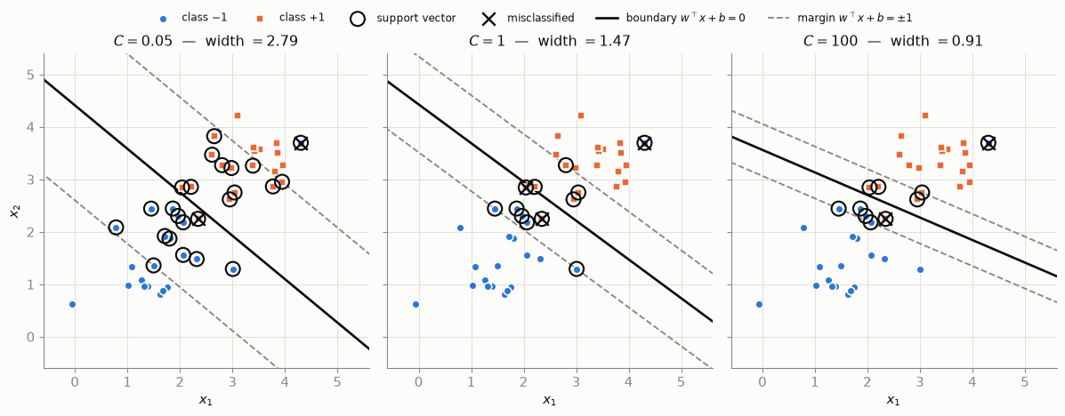
Figure 4: The same non-separable data under three violation prices. Small \(C\) buys a wide corridor and tolerates several points inside it; large \(C\) narrows the band to reduce slack. Ringed points have \(\alpha_i > 0\) (support-vector-like); black × marks misclassified points — the planted outlier at (4.3, 3.7) is lost at every \(C\). Axes are identical across panels.

Read the panels left to right:

  • Small \(C = 0.05\): violations are cheap, so the optimizer keeps \(\lVert w \rVert\) small and the corridor wide, letting a handful of borderline points (and the outlier) sit inside or across it. Many points participate in the solution (\(\alpha_i > 0\)).
  • Medium \(C = 1\): a balance — moderate margin, moderate slack.
  • Large \(C = 100\): every unit of slack is expensive, so the boundary tightens against the training points and the margin band narrows sharply. The fit chases individual observations harder — including reshaping itself around an outlier it still cannot classify.

Neither extreme is “better” in general. Large \(C\) tracks the training data more tightly (risking sensitivity to noise); small \(C\) prioritizes a wide margin (risking underfit if genuine structure is sacrificed). On held-out data the best \(C\) is an empirical question — typically settled by cross-validation, which is deliberately out of scope for this geometric tour.

7.3 Soft margins revive non-uniqueness

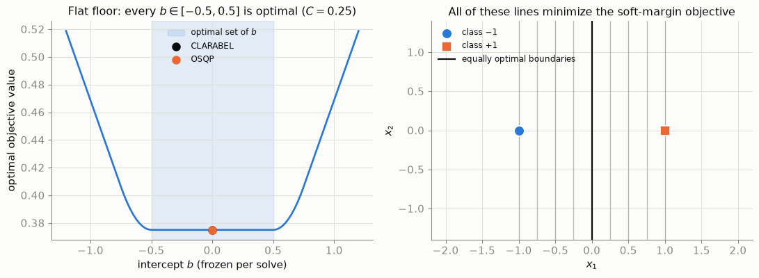
Section 5 promised a genuine two-class example where the intercept is non-unique. The soft-margin problem delivers one, because the hinge penalty can go flat in \(b\). Take the minimal dataset \(x_- = (-1, 0)\) with \(y = -1\) and \(x_+ = (+1, 0)\) with \(y = +1\), and a small price \(C = 0.25 < \tfrac12\). Working through the objective \(\tfrac12 w_1^2 + C\big[\max(0, 1 - w_1 - b) + \max(0, 1 - w_1 + b)\big]\): while both points violate the margin, the two hinge terms consume \(b\) in opposite directions and it cancels exactly, leaving \(\tfrac12 w_1^2 + 2C(1 - w_1)\), minimized at \(w_1 = 2C = 0.5\). The result: \(w^\star = (0.5, 0)\) is unique, but every \(b \in [-0.5, +0.5]\) is optimal, with identical objective value \(0.375\). The decision boundary \(x_1 = -2b\) can sit anywhere in \([-1, 1]\) — anywhere between the two data points, endpoints included. The optimizer is genuinely indifferent:

Flat-b demonstration: solver disagreement + objective scan
X_flat = np.array([[-1.0, 0.0], [1.0, 0.0]])
y_flat = np.array([-1, +1])
C_flat = 0.25

sol_a = solve_soft(X_flat, y_flat, C_flat, solver=cp.CLARABEL)
sol_b = solve_soft(X_flat, y_flat, C_flat, solver=cp.OSQP)
print(f"CLARABEL: w = ({sol_a['w'][0]:.4f}, {sol_a['w'][1]:.4f}), "
      f"b = {sol_a['b']:+.4f}, objective = {sol_a['obj']:.6f}")
print(f"OSQP    : w = ({sol_b['w'][0]:.4f}, {sol_b['w'][1]:.4f}), "
      f"b = {sol_b['b']:+.4f}, objective = {sol_b['obj']:.6f}")
assert abs(sol_a["obj"] - sol_b["obj"]) < 1e-5      # same optimal value...
assert np.allclose(sol_a["w"], sol_b["w"], atol=1e-3)  # ...same w*

# scan: freeze b, minimize over (w, ξ) — the floor of this curve is the optimal set
b_grid = np.linspace(-1.2, 1.2, 97)
obj_b = []
for b_fix in b_grid:
    w_, xi_ = cp.Variable(2), cp.Variable(2)
    p = cp.Problem(
        cp.Minimize(0.5 * cp.sum_squares(w_) + C_flat * cp.sum(xi_)),
        [cp.multiply(y_flat, X_flat @ w_ + b_fix) >= 1 - xi_, xi_ >= 0])
    p.solve(solver=cp.CLARABEL)
    obj_b.append(p.value)
obj_b = np.array(obj_b)
flat = np.abs(b_grid) <= 0.5
assert obj_b[flat].max() - obj_b[flat].min() < 1e-6   # exactly flat inside
assert obj_b[np.abs(b_grid) > 0.55].min() > obj_b[flat].max() + 1e-4

fig, (axL, axR) = plt.subplots(1, 2, figsize=(11.5, 4.3))
axL.plot(b_grid, obj_b, color=BLUE, lw=2)
axL.axvspan(-0.5, 0.5, color="#2a78d61f", label=r"optimal set of $b$")
for sol, name, c in [(sol_a, "CLARABEL", INK), (sol_b, "OSQP", ORANGE)]:
    axL.scatter([sol["b"]], [sol["obj"]], s=70, c=c, zorder=5, label=name)
axL.set_xlabel("intercept $b$ (frozen per solve)")
axL.set_ylabel("optimal objective value")
axL.legend(frameon=False, fontsize=9)
axL.set_title(rf"Flat floor: every $b\in[-0.5,0.5]$ is optimal ($C={C_flat}$)")

scatter_classes(axR, X_flat, y_flat, s=120)
for b_show in np.linspace(-0.5, 0.5, 9):
    axR.axvline(-2 * b_show, color=MUTED, lw=1.0, alpha=0.55)
axR.axvline(0, color=INK, lw=1.6, label="equally optimal boundaries")
axR.set_xlim(-2.2, 2.2); axR.set_ylim(-1.4, 1.4)
axR.set_xlabel("$x_1$"); axR.set_ylabel("$x_2$")
axR.legend(frameon=False, fontsize=9, loc="upper left")
axR.set_title("All of these lines minimize the soft-margin objective")
plt.tight_layout()
plt.show()
CLARABEL: w = (0.5000, 0.0000), b = +0.0000, objective = 0.375000
OSQP    : w = (0.5000, 0.0000), b = -0.0000, objective = 0.375000
Figure 5: A valid two-class case with a non-unique intercept. Left: the optimal objective as a function of \(b\) (each dot is a full CVXPY solve with \(b\) frozen) is exactly flat on \([-0.5, 0.5]\); two solvers pick different points on the flat floor. Right: the corresponding band of equally optimal decision boundaries — the normal vector is pinned, the position is not.

To be precise about which quantity is non-unique here: \(w^\star\) is unique (strict convexity in \(w\) never lets go), the optimal objective value is unique (it always is, for a convex problem), but the intercept — and with it the position of the decision boundary — is an entire interval. Convexity guarantees the set of optima is convex (here, a line segment in \((w, b)\)-space); it never promised a single point. This flat-\(b\) phenomenon is a recognized property of soft-margin SVMs at small \(C\) (analyzed in detail by Burges & Crisp, Uniqueness of the SVM Solution, NeurIPS 1999), not a solver artifact — which is exactly what the two-solver disagreement on a shared flat floor shows.

8 Numerical verification and interpretation

A compact audit of every claim, in one place. For the hard-margin fit, all constraints must hold with functional margin at least \(1\); for the soft-margin fits, the relaxed constraints \(y_i f(x_i) + \xi_i \ge 1\) must hold, with the slack doing exactly the work the plots show:

Constraint audits for all solved problems
print(f"tolerance used in all checks: {TOL:g}\n")
print("hard margin (Dataset A):")
print(f"  min_i  y_i(w·x_i + b)          = {func_margins.min():.10f}  ≥ 1 − tol ✓")

print("\nsoft margin (Dataset B):")
for f in fits:
    resid = y_B * (X_B @ f["w"] + f["b"]) + f["xi"]
    print(f"  C = {f['C']:>6g}:  min_i [y_i(w·x_i+b) + ξ_i] = "
          f"{resid.min():.10f}  ≥ 1 − tol ✓,   min ξ_i = {f['xi'].min():.1e} ≥ 0 ✓")
    assert resid.min() >= 1 - 1e-5 and f["xi"].min() >= -TOL
tolerance used in all checks: 1e-06

hard margin (Dataset A):
  min_i  y_i(w·x_i + b)          = 1.0000000001  ≥ 1 − tol ✓

soft margin (Dataset B):
  C =   0.05:  min_i [y_i(w·x_i+b) + ξ_i] = 0.9999999963  ≥ 1 − tol ✓,   min ξ_i = 0.0e+00 ≥ 0 ✓
  C =      1:  min_i [y_i(w·x_i+b) + ξ_i] = 0.9999999945  ≥ 1 − tol ✓,   min ξ_i = 0.0e+00 ≥ 0 ✓
  C =    100:  min_i [y_i(w·x_i+b) + ξ_i] = 0.9999999998  ≥ 1 − tol ✓,   min ξ_i = 0.0e+00 ≥ 0 ✓

The slack values connect directly back to Figure 4: points printed as violations are precisely the ringed-or-crossed points drawn inside or across each panel’s margin band, and each panel’s \({\sum_i \xi_i}\) shrinks as \(C\) grows while its band narrows.

As a final sanity check, scikit-learn’s SVC — an independent implementation solving the dual with a specialized algorithm (SMO), rather than our primal QP — should land on the same hyperplanes:

Cross-check against scikit-learn (optional, not the primary solve)
from sklearn.svm import SVC

svc_hard = SVC(kernel="linear", C=1e8, tol=1e-8).fit(X_A, y_A)  # huge C ≈ hard margin
print("hard   : sklearn w =", np.round(svc_hard.coef_[0], 6),
      " b =", np.round(svc_hard.intercept_[0], 6))
assert np.allclose(svc_hard.coef_[0], w_hard, atol=1e-4)
assert abs(svc_hard.intercept_[0] - b_hard) < 1e-4

for f in fits:
    svc = SVC(kernel="linear", C=f["C"], tol=1e-8).fit(X_B, y_B)
    dw = np.linalg.norm(svc.coef_[0] - f["w"])
    db = abs(svc.intercept_[0] - f["b"])
    print(f"C={f['C']:>6g}: sklearn w = {np.round(svc.coef_[0], 4)}, "
          f"b = {svc.intercept_[0]:+.4f}   (‖Δw‖ = {dw:.1e}, |Δb| = {db:.1e})")
    assert dw < 1e-3 and db < 1e-3
hard   : sklearn w = [0.5 0.5]  b = -2.0
C=  0.05: sklearn w = [0.4575 0.5523], b = -2.4371   (‖Δw‖ = 5.0e-08, |Δb| = 1.6e-07)
C=     1: sklearn w = [0.8088 1.0946], b = -4.8491   (‖Δw‖ = 5.3e-07, |Δb| = 1.5e-06)
C=   100: sklearn w = [0.8676 2.0191], b = -7.1951   (‖Δw‖ = 1.8e-04, |Δb| = 4.2e-04)

Same \(w\), same \(b\), to solver tolerance, on every problem — two independent code paths agreeing on the unique optimum that convexity promised.

Fitting an SVM is solving an optimization problem, but understanding what the fit did requires holding four views of the same object at once:

  • geometry in input space — a boundary, a band, and points that touch it;
  • feasibility and objective in parameter space — each data point is a half-space constraint on \((w, b)\), and the optimum is where the shrinking norm ball last touches the feasible set (Figure 3);
  • support vectors / active constraints — the sparse subset of data with \(\alpha_i > 0\) that actually holds the solution in place;
  • the regularization trade-off\(C\) pricing margin width against violations, with neither extreme universally right.

9 Common misconceptions

A closing checklist of traps this post was built to disarm:

  1. “Any separating line is equally good.” All separators achieve 100% training accuracy, but they differ enormously in clearance (Figure 1: \(\gamma = 1.414\) vs \(0.86\)). The max-margin criterion is precisely a principled tiebreaker among them.
  2. “Convex means the answer must be unique.” Convexity eliminates bad local minima; it says nothing about a unique minimizer. We exhibited a genuine two-class problem whose optimal intercepts form an interval (Figure 5). Uniqueness needs extra conditions — strict convexity in all variables, or the two-class separable structure of Section 5.
  3. “The margin is the distance from the boundary to a support vector.” That is the one-sided geometric margin \(1/\lVert w \rVert\). The margin band — the full empty street the SVM maximizes — is twice that, \(2/\lVert w \rVert\) (both are drawn in Figure 2).
  4. “Larger \(C\) always gives a better classifier.” Larger \(C\) only penalizes training violations more heavily. On Dataset B it progressively contorts the fit around an outlier that no linear boundary can classify, narrowing the margin band substantially (see the widths printed in each panel of Figure 4) without ever fixing the outlier. Training-set obedience is not generalization.
  5. “The solver found a solution, so one always exists.” Hard-margin feasibility is an assumption about the data, not a gift of convexity — on our overlapping dataset the solver correctly returned infeasible, and slack variables had to be invented before any answer existed at all.