Tensor Inverses in Practice

Four real problems where the operator is a tensor. For each one, this post names the product that applies, takes the inverse in that product, and measures what flattening the tensor into a matrix would have cost.

Two earlier posts give the background. Tensor Factorizations and Tensor Inverses has the algebra. Uses of Tensor Factorizations has the compression case. The first one shows that a tensor has no default product. Because of that, it has no default inverse either.

This post answers the question that leaves open. For a given problem, which product applies, and what does flattening cost?

The table of inverses comes first. Then the four problems. Then all the numbers side by side.

1 Words used here

Some of these words have a different everyday meaning. This is what they mean in this post.

Mode. One axis of an array. A \(52\times24\times8\) array has three modes.
Order. How many modes an array has. A vector has order 1, a matrix order 2.
Frontal slice. For a three-mode array \(\mathcal{A}\), the matrix \(\mathcal{A}[:,:,k]\). There is one for each value of \(k\).
Flatten. Rearrange a tensor into a matrix or a vector. Other papers say unfold or vectorise for the same idea. This post says flatten throughout.
Operator. Anything that takes an input and returns an output. Here it is usually a tensor that takes a tensor and returns a tensor.
Rank. How many independent directions an operator really uses. An operator on nine dimensions can have rank 6.
Null space. The set of inputs that an operator sends to zero. An operator with a null space larger than \(\{0\}\) has no inverse.
Inverse. The operator that undoes another operator.
Pseudoinverse. What you use when no inverse exists. It undoes the operator on the directions the operator keeps, and returns zero on the directions the operator destroys.
Condition number, \(\kappa\). How much an operator can magnify an error. If \(\kappa = 10^{12}\), an error in the twelfth digit of the input can reach the first digit of the output.
Residual. How far a computed answer sits from the answer it should give.
Covariance. A table saying how strongly each pair of measurements moves together.
Precision matrix. The inverse of a covariance matrix. Here the word does not mean accuracy.

2 The kinds of tensor inverse

A matrix inverse undoes matrix multiplication. There is one matrix product, so there is one matrix inverse.

Tensors work differently. There are several tensor products, and each one has its own inverse. You cannot use one in place of another, and none of them is the tensor inverse.

Inverse	Product it inverts	Order and shape it needs	Reach for it when	What it costs
Mode-\(n\) pseudoinverse	mode-\(n\) product \(\times_n\)	any order	you want to recover a factor, a mixing matrix, or a change of basis along one mode: \(A = Y_{(n)}X_{(n)}^{\dagger}\)	it inverts a matrix that acts on one mode. It does not invert the tensor. Readers confuse these two more often than anything else in this table
t-inverse / t-pseudoinverse	t-product \(*\)	third order, with a meaningful third mode	the third mode is time, wavelength, or a frequency grid: video, hyperspectral cubes, some fMRI layouts	one FFT along mode 3, then \(n_3\) matrix inverses. Each slice is inverted on its own, so a single bad slice ruins the whole answer
Einstein-product inverse	Einstein product \(\circledast\)	even order, square: \(I_1{\times}\cdots{\times}I_N{\times}I_1{\times}\cdots{\times}I_N\)	the tensor really is a linear map that takes a tensor and returns one: stiffness and compliance, or a PDE written out on a grid	it is the same object as a \((\prod_k I_k)^2\) matrix, and it exists exactly when that matrix can be inverted
Multilinear Moore–Penrose	Einstein product	even order, rectangular or rank-deficient	same setting, but the operator is not square or not full rank	the one object that satisfies the four Penrose conditions; at order 2 it is the ordinary matrix pseudoinverse
Tucker- or TT-format inverse	mode products, TT contraction	any order, low multilinear or TT rank	the full operator will not fit in memory, and you need the inverse stored in the same compressed form	only approximate. The inverse usually needs a higher rank than the operator
CP-based approximate inverse	—	any order	a rough, cheap approximation is enough and you never need the exact inverse	nothing guarantees that it exists or that it is unique. Treat it as an approximation, not an inverse
Kronecker-separable precision	—	any order	you are modelling a covariance over a multi-way array (the tensor-normal or matrix-normal model)	not a tensor inverse at all. You are assuming that the inverse splits mode by mode. It is in this table because people mistake it for one

2.1 Two rules that come with the table

In real work you solve, you do not invert. This is the same rule as for matrices. Tensor Krylov methods, such as t-product GMRES, find \(\mathcal{X}\) in \(\mathcal{A} * \mathcal{X} = \mathcal{B}\) without ever building \(\mathcal{A}^{-1}\) (El Guide et al. 2021). This post builds the inverse anyway, so that you can see what it looks like. That is a choice made for teaching, not advice for production code.

Using the wrong product is a mistake of kind, not a mistake of accuracy. Suppose \(\lVert \mathcal{A} \times_n \mathcal{X} - \mathcal{B}\rVert\) comes out small. That tells you nothing about \(\mathcal{A} * \mathcal{X} = \mathcal{B}\). The two products multiply along different modes. They are different equations that happen to use the same letters. Computing in higher precision will never turn one into the other.

3 Data

Four problems and four sources. Two are downloaded. One is a set of published material constants. One is simulated, because the real data needs a signed agreement.

3.1 An off-axis carbon/epoxy ply

What it is. Five elastic constants for a unidirectional T300/5208 carbon-fibre/epoxy ply at room temperature: \(E_1 = 181\) GPa along the fibres, \(E_2 = 10.3\) GPa across them, \(G_{12} = 7.17\) GPa, \(\nu_{12} = 0.28\), \(\nu_{23} = 0.35\). These are typical published values for that material, written out in full so you can check the arithmetic below. Nothing here turns on the third significant figure.
Who measures them and why. Materials labs pull, press and twist small test pieces cut from cured panels. Structural engineers use the results to predict how a part will bend before anyone builds it. The measurement exists to feed a stiffness model.
What this post asks of them. Build the fourth-order stiffness tensor and rotate the ply \(30°\) off the fibre axis. Then invert it to get compliance, so that a known stress returns the strain it caused.
What being wrong costs. Compliance turns a load into a deflection. An error here means an aircraft panel or a pressure vessel is sized against the wrong strain. That is a part that breaks, not a plot that looks wrong.
Why a tensor inverse. A \(3\times3\times3\times3\) stiffness tensor really is a linear map. It takes a symmetric \(3\times3\) matrix and returns a symmetric \(3\times3\) matrix. This is exactly what the Einstein product describes. It is also the one problem here where flattening works, so it is a fair place to start.

3.2 Pavia University

Provenance. A hyperspectral image of the University of Pavia campus in northern Italy, \(610\times340\) pixels over 103 spectral bands at 1.3 m ground resolution. The ROSIS sensor recorded it from an aircraft. Prof. Paolo Gamba released it for research; he works at the Telecommunications and Remote Sensing Laboratory at the University of Pavia. Graña, Veganzones and Ayerdi at UPV/EHU then put it into the Hyperspectral Remote Sensing Scenes collection, which serves it today.
Collector and motive. An aircraft flight, not a survey and not a web scrape. The team flew the scene and released it so that hyperspectral classification methods would share one benchmark. Hundreds of remote-sensing papers now use it.
What this post uses. A \(128\times128\times103\) crop. src/fetch_data.py writes it to data/paviaU_crop.npz, which is committed. The official host blocks scripted downloads, so the script takes the whole scene from an open mirror, cuts out the crop, and throws the rest away.
What this post asks of it. Blur the cube with an operator that smears space and mixes neighbouring bands, then try to get it back two ways.
What being wrong costs. Hyperspectral analysis identifies a material from the shape of a pixel’s spectrum. Suppose a method sharpens the picture but leaves the bands mixed. It then reports the wrong material, and reports it with confidence. A mineral survey, a crop-disease map or a pollution estimate would rest on a spectrum that belongs to no real material.
Why a tensor inverse. The blur mixes the bands into each other. You therefore cannot treat each band as a separate problem. The t-product is built for this case: a third mode whose order means something, and slices that mix.

3.3 A synthetic four-dimensional scan

It is synthetic, and this is how it is made. A \(16\times16\times16\times120\) array. There are four regressors: a constant, two on-off task blocks with different periods, and a slow linear drift. Each regressor has its own Gaussian blob somewhere in space. The array is the design matrix times those blobs, plus independent Gaussian noise with \(\sigma = 0.4\). The random seed is 7.
What it stands in for, and why it is simulated. A task-fMRI session of the kind in ADNI or the CMU StarPlus set. Those need an application and a signed agreement, so a render cannot download them. There is a better reason too. This section has to recover a map that it already knows, so that it can score the result. No real scan comes with the answer attached.
What being wrong costs. A task map that puts activity in the wrong voxels becomes a published claim about which part of the brain does a job. The claim would be wrong.
Why a mode-\(n\) pseudoinverse. Time is one mode out of four, and the design matrix acts only on that mode. Regress along that mode, treating the three space modes as samples, and the whole solve is \(120\times4\). The alternative is written out below.

3.4 Chicago incident counts

Provenance. The City of Chicago open data portal, “Crimes — 2001 to Present” (Socrata resource ijzp-q8t2), a public extract of the police department’s records-management system.
Collector and motive. Officers of the Chicago Police Department enter each reported incident, and the city publishes the records under its open-data programme. These are reports, not offences. How often people report a crime varies by area and by offence type, and the portal says so.
What this post uses. All of 2023, for community areas 1–24 and the eight most common offence types. The counts go into a \(52 \times 24 \times 8\) array: week by area by offence type. The bins are 52 whole weeks. The one leftover day of the year is thrown away, so that the last bin is not longer than the others. src/fetch_data.py writes the array to data/chicago_counts.npz, which is committed, so a render never calls the API. The cell below prints the incident count.
What this post asks of it. Estimate the covariance of the weekly array. A forecast needs that covariance before it can give any error bars.
What being wrong costs. Cities use covariance estimates to plan patrols and staffing. A model that is confident about the wrong areas sends officers to the wrong areas.
Why a structured inverse. Flattened, one week is a 192-dimensional vector, and there are only 52 weeks. The full covariance therefore cannot be inverted. A precision matrix that splits mode by mode can be fitted from the same data. As that section explains, splitting it is an assumption you are making, not an inverse you are taking.

4 Compliance: the Einstein product

Who does this. A mechanical engineer setting up a finite-element run on an anisotropic laminate.

flowchart LR
  S["<b>σ</b><br/>stress, 3 × 3"] --> C["<b>ℂ</b><br/>stiffness<br/>3 × 3 × 3 × 3"]
  C -->|"invert under ⊛"| SS["<b>𝕊 = ℂ<sup>+</sup></b><br/>compliance"]
  SS --> E["<b>ε = 𝕊 ⊛ σ</b><br/>strain, 3 × 3"]

Figure 1: Stress in, strain out. The operator is a fourth-order stiffness tensor, and the inverse is taken under the Einstein product.

Hooke’s law in tensor form is \(\sigma_{ij} = \mathbb{C}_{ijkl}\varepsilon_{kl}\). Summing over the last two indices of \(\mathbb{C}\) against a \(3\times3\) matrix is the Einstein product.

So \(\mathbb{C}\) takes a \(3\times3\) matrix and returns a \(3\times3\) matrix. Compliance is the operator that undoes it.

Build the ply, rotate it \(30°\) off the fibre axis, and look at the operator as a \(9\times9\) matrix.

Code

C4 = D.off_axis_stiffness(30.0)
flat = C4.reshape(9, 9)
sv = np.linalg.svd(flat, compute_uv=False)

print(f"stiffness tensor  {C4.shape}, as an operator {flat.shape}")
print("singular values / largest:")
print(np.array2string(sv / sv.max(), precision=6, suppress_small=False))
print(f"rank {np.linalg.matrix_rank(flat)} of 9")

stiffness tensor  (3, 3, 3, 3), as an operator (9, 9)
singular values / largest:
[1.000000e+00 8.611932e-02 7.803630e-02 7.803630e-02 4.151939e-02
 4.151939e-02 3.926067e-18 7.338246e-19 2.957319e-19]
rank 6 of 9

Three of the nine singular values are zero, to machine precision. So the stiffness tensor is a \(9\times9\) operator of rank 6, not rank 9. The Einstein-product inverse does not exist.

Code

try:
    T.einstein_inv(C4, 2)
except np.linalg.LinAlgError as err:
    print(f"einstein_inv: {err}")

einstein_inv: Singular matrix

This is not a flaw in the material. It follows from the minor symmetries \(\mathbb{C}_{ijkl} = \mathbb{C}_{jikl} = \mathbb{C}_{ijlk}\). Those symmetries mean the operator ignores the antisymmetric part of its input, and never produces one.

The antisymmetric \(3\times3\) matrices fill three dimensions. Those three are the null space. This makes physical sense: turning a rigid body does not stretch it.

The object that does exist is the multilinear Moore–Penrose inverse, which is row 4 of the table rather than row 3. It undoes the map on the six symmetric directions, and returns zero on the other three.

Code

S4 = T.einstein_pinv(C4, 2)
sigma = D.applied_stress()
eps = T.einstein(S4, sigma, 2)
back = T.einstein(C4, eps, 2)

print("applied stress (MPa)")
print(np.array2string(sigma / 1e6, precision=1, suppress_small=True))
print("\nrecovered strain (x 1e-3)")
print(np.array2string(eps * 1e3, precision=4, suppress_small=True))
print(f"\nstrain is symmetric: {np.allclose(eps, eps.T)}")
print(f"round trip C(eps) vs sigma, relative error: {np.linalg.norm(back - sigma) / np.linalg.norm(sigma):.2e}")

applied stress (MPa)
[[120.  54.   0.]
 [ 54.  42.   0.]
 [  0.   0.   0.]]

recovered strain (x 1e-3)
[[ 1.303  -0.4146  0.    ]
 [-0.4146  0.6906 -0.    ]
 [ 0.     -0.     -0.7285]]

strain is symmetric: True
round trip C(eps) vs sigma, relative error: 5.32e-16

The strain comes back symmetric, and the round trip closes to machine precision.

Notice the shear–extension coupling. A ply turned by \(30°\) under mostly normal stress also picks up a negative shear strain. Engineers stack plies in balanced pairs so that these shear strains cancel.

4.1 Why Voigt notation is a flattening that works

Voigt notation stacks the six independent components of a symmetric \(3\times3\) tensor into a vector of length 6. That turns \(\mathbb{C}\) into a \(6\times6\) matrix. It is a flattening, it is standard engineering practice, and here it is exactly right.

The rank count above explains why. The three directions that Voigt throws away are exactly the three in the null space. Flattening onto the symmetric directions loses nothing, because there was nothing there to lose.

Code

C6 = D.tensor_to_voigt_stiffness(C4)
S6 = np.linalg.inv(C6)
S4_from_voigt = D.compliance_to_tensor(S6, reuter=True)

print(f"Voigt stiffness 6x6: rank {np.linalg.matrix_rank(C6)}, condition number {np.linalg.cond(C6):.1f}")
print(f"max |S4_from_voigt - S4|: {np.abs(S4_from_voigt - S4).max():.2e}")

Voigt stiffness 6x6: rank 6, condition number 39.9
max |S4_from_voigt - S4|: 1.42e-25

The Voigt matrix is well conditioned and full rank, and it matches the multilinear pseudoinverse to the last digit.

Flattening is not the problem. Flattening along the wrong structure is the problem.

4.2 The mistake Voigt still lets you make

Voigt compliance uses engineering shear strains, \(\gamma_{12} = 2\varepsilon_{12}\). The tensor uses \(\varepsilon_{12}\) instead. So converting the inverted \(6\times6\) back to a fourth-order tensor needs Reuter’s factors: divide by 2 for each shear index. Skip them and the shear terms come out 2 or 4 times too large.

Code

bad = D.compliance_to_tensor(S6, reuter=False)
eps_bad = T.einstein(bad, sigma, 2)
err_bad = np.linalg.norm(T.einstein(C4, eps_bad, 2) - sigma) / np.linalg.norm(sigma)

print("strain without Reuter factors (x 1e-3)")
print(np.array2string(eps_bad * 1e3, precision=4, suppress_small=True))
print(f"\nshear  ratio to correct: {eps_bad[0, 1] / eps[0, 1]:+.2f}")
print(f"normal ratio to correct: {eps_bad[0, 0] / eps[0, 0]:+.2f}")
print(f"round-trip relative error: {err_bad:.2f}")

strain without Reuter factors (x 1e-3)
[[-1.2328  5.3348  0.    ]
 [ 5.3348 -1.0556  0.    ]
 [ 0.      0.      0.7883]]

shear  ratio to correct: -12.87
normal ratio to correct: -0.95
round-trip relative error: 3.16

When the ply is turned off-axis, the error is not limited to shear. Turning the ply puts shear–extension terms into the compliance. If their scale is wrong, the error spreads through the whole solve. The normal strains then flip sign, and the round trip is wrong by more than 300%.

On the fibre axis those coupling terms are zero. The same mistake then makes the shear exactly 4 times too large, and leaves everything else correct.

Code

C4_0 = D.off_axis_stiffness(0.0)
eps_0 = T.einstein(T.einstein_pinv(C4_0, 2), sigma, 2)
S6_0 = np.linalg.inv(D.tensor_to_voigt_stiffness(C4_0))
bad_0 = T.einstein(D.compliance_to_tensor(S6_0, reuter=False), sigma, 2)

print(f"on-axis shear  ratio: {bad_0[0, 1] / eps_0[0, 1]:.3f}")
print(f"on-axis normal ratio: {bad_0[0, 0] / eps_0[0, 0]:.3f}")

on-axis shear  ratio: 4.000
on-axis normal ratio: 1.000

The pseudoinverse cannot make this mistake, because it never leaves the tensor. So there is a trade. Flattening gives you a smaller, better-behaved object. In exchange, you must apply a conversion rule by hand, and apply it correctly.

5 Hyperspectral restoration: the t-product

Who does this. A remote-sensing analyst deblurring a data cube before classifying it.

flowchart LR
  X["<b>𝒳</b><br/>clean cube<br/>128 × 128 × 103"] --> A["<b>𝒜</b><br/>blur operator<br/>smear + band leak"]
  A --> B["<b>ℬ = 𝒜 * 𝒳</b><br/>observed"]
  B --> F["band-by-band<br/>invert slice 0 only"]
  B --> TP["t-solve<br/>all 103 Fourier slices"]
  F --> R1["spatially sharp,<br/>spectrally still mixed"]
  TP --> R2["<b>𝒳̂</b>"]

Figure 2: One t-solve against 103 separate 2D deblurring problems. The flattening keeps only the first frontal slice, and the band mixing lives in the ones it drops.

The blur has two parts. The optics smear each band across space. The sensor also leaks signal between neighbouring wavelengths.

Under the t-product both parts fit into one operator \(\mathcal{A}\). Frontal slice 0 holds the spatial smear, and slices \(\pm 1\) hold the leak.

Code

cube, meta = D.pavia_crop()
n, bands = cube.shape[0], cube.shape[2]
LEAK = 0.12
A = D.blur_operator(n, bands, width=1.4, leak=LEAK)

rng = np.random.default_rng(T.SEED)
observed = T.tprod(A, cube)
observed = observed + rng.normal(0, 1e-3 * observed.std(), observed.shape)

print(f"crop {cube.shape} from the {tuple(meta['full_shape'])} scene at origin {meta['origin']}")
print(f"operator {A.shape}: spatial smear in slice 0, {LEAK:.0%} band leak in slices 1 and -1")
print(f"operator as a tensor:            {A.nbytes / 1e6:6.1f} MB")
print(f"same operator flattened to a matrix:      {(n * bands) ** 2 * 8 / 1e9:6.1f} GB")

crop (128, 128, 103) from the (610, 340, 103) scene at origin [150, 100]
operator (128, 128, 103): spatial smear in slice 0, 12% band leak in slices 1 and -1
operator as a tensor:              13.5 MB
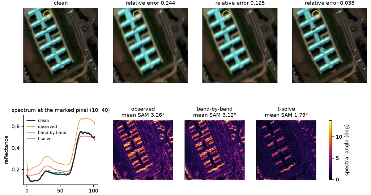
same operator flattened to a matrix:         1.4 GB

Two methods are compared below. Band-by-band deblurs each of the 103 bands on its own, which is the flattening. t-solve solves the whole cube at once in the t-product.

Undoing a blur is unstable. A small amount of noise in the input becomes a large amount of noise in the answer.

Both methods therefore get the same Tikhonov damping, and each one picks the \(\lambda\) that suits it best. This is generous to the flattening. It also leaves the band mixing as the only real difference between the two methods.

Code

def relative(x):
    return np.linalg.norm(x - cube) / np.linalg.norm(cube)


lambdas = np.logspace(-6, 1, 15)
results = {}
for name, solver in (
    ("band-by-band", T.band_by_band_solve),
    ("t-solve", T.treg_solve),
):
    err, lam = min((relative(solver(A, observed, l)), l) for l in lambdas)
    start = time.perf_counter()
    recovered = solver(A, observed, lam)
    results[name] = {
        "cube": recovered,
        "lam": lam,
        "rel": err,
        "sam": float(D.spectral_angle(cube, recovered).mean()),
        "secs": time.perf_counter() - start,
    }

header = f"{'':<13} {'lambda':>8} {'rel error':>10} {'mean SAM':>9} {'seconds':>8}"
print(header)
print("-" * len(header))
print(f"{'observed':<13} {'':>8} {relative(observed):10.4f} "
      f"{D.spectral_angle(cube, observed).mean():8.2f}° {'':>8}")
for name, r in results.items():
    print(f"{name:<13} {r['lam']:8.0e} {r['rel']:10.4f} {r['sam']:8.2f}° {r['secs']:8.2f}")

                lambda  rel error  mean SAM  seconds
----------------------------------------------------
observed                   0.2444     3.26°         
band-by-band     3e-01     0.1247     3.12°     0.06
t-solve          1e-04     0.0376     1.79°     0.14

Band-by-band deblurring halves the relative error and then stops improving. Its best \(\lambda\) sits at the smoothest end of the grid. A method chooses heavy smoothing when it cannot fix the real problem. Here the real problem is the band mixing, which this method threw away.

The t-solve gets about three times closer. The spectral angle also drops by 40%. Spectral angle is the measure that decides which material a pixel contains, so that is the number that matters.

Code

def rgb(c):
    im = np.stack([c[:, :, 46], c[:, :, 27], c[:, :, 10]], axis=-1)
    lo, hi = np.percentile(im, [1, 99])
    return np.clip((im - lo) / (hi - lo), 0, 1)


recovered = {k: results[k]["cube"] for k in results}
sam = {
    name: D.spectral_angle(cube, data).reshape(n, n)
    for name, data in [("observed", observed), *recovered.items()]
}

# Mark a pixel where the two methods actually disagree, rather than an
# arbitrary one: the 97th percentile of the band-by-band minus t-solve gap,
# taken away from the border so the marker is not clipped.
gap = sam["band-by-band"] - sam["t-solve"]
interior = np.zeros_like(gap, dtype=bool)
interior[8:-8, 8:-8] = True
# argsort puts the masked-out border pixels first, so index from the top.
ranked = np.argsort(np.where(interior, gap, -np.inf).ravel())
px, py = np.unravel_index(ranked[-1 - int(0.03 * interior.sum())], (n, n))

fig, axes = plt.subplots(2, 4, figsize=(11, 6.0), height_ratios=[1.35, 1])
fig.subplots_adjust(hspace=0.28)
for ax, (name, data) in zip(
    axes[0], [("clean", cube), ("observed", observed), *recovered.items()]
):
    ax.imshow(rgb(data))
    title = name if name == "clean" else f"{name}\nrelative error {relative(data):.3f}"
    ax.set_title(title)
    ax.plot(py, px, "o", mfc="none", mec=GOLD, mew=1.8, ms=13)
    ax.set_xticks([])
    ax.set_yticks([])

spec = axes[1][0]
spec.plot(cube[px, py, :], color=INK, lw=2.0, label="clean", zorder=3)
spec.plot(observed[px, py, :], color=GOLD, lw=1.2, label="observed")
spec.plot(recovered["band-by-band"][px, py, :], color=CORAL, lw=1.3, label="band-by-band")
spec.plot(recovered["t-solve"][px, py, :], color=TEAL, lw=1.3, label="t-solve")
spec.set_title(f"spectrum at the marked pixel ({px}, {py})")
spec.set_xlabel("band")
spec.set_ylabel("reflectance")
spec.legend(frameon=False, fontsize=7)

vmax = float(np.percentile(sam["observed"], 99))
for ax, name in zip(axes[1][1:], ["observed", "band-by-band", "t-solve"]):
    im = ax.imshow(sam[name], cmap="inferno", vmin=0, vmax=vmax)
    ax.set_title(f"{name}\nmean SAM {sam[name].mean():.2f}°")
    ax.set_xticks([])
    ax.set_yticks([])
fig.colorbar(im, ax=axes[1][1:], shrink=0.85, label="spectral angle (deg)")
plt.show()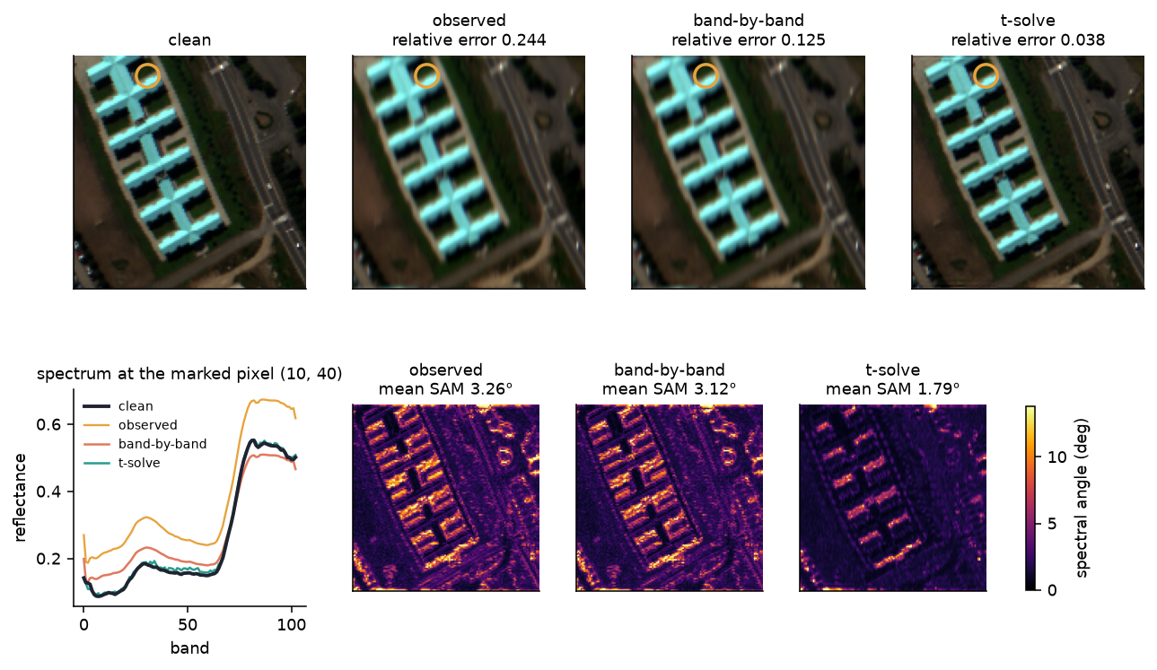

Figure 3: Pavia University, a 128×128 crop. Top: an RGB view built from bands 46, 27 and 10. Bottom left: the spectrum at one marked pixel. Bottom right: the spectral angle at every pixel against the clean cube, all three on one scale. Band-by-band deblurring sharpens the picture but leaves the spectral-angle errors almost as large as in the blurred input. The t-solve reduces them.

The spectra show this most clearly. The band-by-band curve keeps the shape of the clean curve, but it does not sit on top of it. It runs above the truth over some bands and below over others. Every band still carries 12% of each neighbour. The t-solve curve lies on the truth.

The spectral-angle maps show the same result across the whole scene. In the band-by-band map the errors are almost as large as in the blurred input. The largest errors sit on roofs and edges. Neighbouring bands differ most there, so the leak does most damage there. In the t-solve map the errors drop everywhere.

Look at the memory line above as well. The same operator takes 13.5 MB as a tensor and 1.4 GB after flattening into a matrix. So the t-product does more than give a better answer. On the full scene it is the only one of the two that fits in memory.

6 The t-inverse, stage by stage

The t-inverse takes four steps, and each step can be drawn. The widget below goes through them on a small \(8\times8\times6\) tensor, built from the same random seed as the rest of the post.

Stage 2 is the important one. After the FFT along mode 3 the six slices become independent of each other, so one tensor inverse turns into six separate matrix inverses. Next, drag Conditioning to the right. Slice 2 and its conjugate partner slice 4 become singular together. The largest entry of the inverse climbs past 1e11, and the solve error rises to 2.6e6. One bad slice ruins the whole tensor. Now switch the solver to pinv. The pseudoinverse drops the bad direction. The identity check then fails, because A·A⁺ sends that direction to zero instead of leaving it alone — but the solve error falls back to 0.09. That is the trade, and the two numbers disagree for a reason.

The numbers in that note come from the same function that produced the widget’s data, so you can check them here:

Code

for level in (0.0, 0.5, 1.0):
    row = []
    for solver in ("inv", "pinv"):
        s = T.widget_state(level, solver)
        row.append((solver, s["residual"], s["max_abs"], s["solve_error"]))
    kappa = T.widget_state(level, "inv")["conds"][2]
    print(f"conditioning {level:.1f}   kappa(slice 2) = {kappa:.2e}")
    for solver, res, mx, solve in row:
        print(f"    {solver:>4}  identity residual {res:8.2e}   max|X| {mx:8.2e}   solve error {solve:8.2e}")

conditioning 0.0   kappa(slice 2) = 6.93e+00
     inv  identity residual 5.31e-16   max|X| 5.67e-01   solve error 1.21e-05
    pinv  identity residual 1.44e-15   max|X| 5.67e-01   solve error 1.21e-05
conditioning 0.5   kappa(slice 2) = 6.93e+06
     inv  identity residual 2.11e-10   max|X| 1.67e+05   solve error 2.57e+00
    pinv  identity residual 3.70e-10   max|X| 1.67e+05   solve error 2.57e+00
conditioning 1.0   kappa(slice 2) = 6.92e+12
     inv  identity residual 2.12e-04   max|X| 1.67e+11   solve error 2.57e+06
    pinv  identity residual 2.04e-01   max|X| 5.51e-01   solve error 9.47e-02

Two points.

First, the identity residual and the solve error disagree once the pseudoinverse starts dropping directions. The solve error is the one to read, because it measures the answer you actually wanted.

Second, slices 2 and 4 are a conjugate pair. In a tensor with real entries, one of them cannot become ill-conditioned on its own.

7 Task maps: the mode-\(n\) pseudoinverse

Who does this. A computational neuroscientist mapping a four-dimensional scan onto a task design.

flowchart LR
  Y["<b>𝒴</b><br/>scan<br/>16 × 16 × 16 × 120"] --> U["flatten on mode 4<br/>120 × 4096"]
  X["<b>X</b><br/>design<br/>120 × 4"] --> P["<b>X<sup>†</sup></b><br/>mode-n pseudoinverse"]
  U --> M["<b>B = X<sup>†</sup> 𝒴<sub>(4)</sub></b>"]
  P --> M
  M --> R["coefficient maps<br/>4 × 4096"]

Figure 4: Regression along one mode. Time is mode 4, and the three space modes become columns, so the solve is the size of the design rather than the size of the scan.

Readers misread this row of the table more often than any other. The mode-\(n\) pseudoinverse inverts the design matrix, on one mode. It does not invert the scan. In fact no tensor is inverted here at all.

Code

scan, design, beta_true = D.synthetic_scan()
start = time.perf_counter()
beta_hat = T.mode_pinv_solve(scan, design, 3)
mode_secs = time.perf_counter() - start
truth = beta_true.reshape(design.shape[1], -1)

print(f"scan {scan.shape}, design {design.shape}, solve took {mode_secs * 1e3:.1f} ms")
names = ["intercept", "task A", "task B", "drift"]
for p, name in enumerate(names[1:], start=1):
    corr = np.corrcoef(beta_hat[p], truth[p])[0, 1]
    print(f"  {name:<10} correlation with truth {corr:.3f}")
print(f"  overall relative error {np.linalg.norm(beta_hat - truth) / np.linalg.norm(truth):.3f}")

scan (16, 16, 16, 120), design (120, 4), solve took 0.4 ms
  task A     correlation with truth 0.960
  task B     correlation with truth 0.903
  drift      correlation with truth 0.657
  overall relative error 0.230

The two task maps come back with correlation 0.96 and 0.90 against the truth. The drift map is weaker, which is what you would expect. Over 120 frames, a slow ramp looks much like noise.

Now count the parameters. The mode-\(n\) method solves one \(120\times4\) system, then reuses that solution across all 4,096 voxels.

Code

voxels, frames, params = 16**3, design.shape[0], design.shape[1]
vec_rows, vec_cols = voxels * frames, voxels * params

print(f"mode-n:  solve is {frames} x {params}, estimates {params * voxels:,} coefficients")
print(f"flattened GLM design matrix: {vec_rows:,} x {vec_cols:,}")
print(f"  = {vec_rows * vec_cols:.2e} entries = {vec_rows * vec_cols * 8 / 1e9:.1f} GB")

mode-n:  solve is 120 x 4, estimates 16,384 coefficients
flattened GLM design matrix: 491,520 x 16,384
  = 8.05e+09 entries = 64.4 GB

The estimates are identical, and the design matrix is 64 GB. That matrix is the same \(120\times4\) block repeated 4,096 times along a diagonal. The mode-\(n\) pseudoinverse is what you get once you notice the repetition and stop writing the copies down.

Code

maps = beta_hat.reshape(beta_true.shape)
fig, axes = plt.subplots(2, 3, figsize=(10, 4.4))
slices = [(1, 8), (2, 7), (3, 8)]
for col, (p, z) in enumerate(slices):
    vmax = float(np.abs(beta_true[p]).max())
    axes[0, col].imshow(beta_true[p][:, :, z], cmap="magma", vmin=0, vmax=vmax)
    axes[1, col].imshow(maps[p][:, :, z], cmap="magma", vmin=0, vmax=vmax)
    corr = np.corrcoef(beta_hat[p], truth[p])[0, 1]
    axes[0, col].set_title(f"{names[p]} — truth")
    axes[1, col].set_title(f"recovered, r = {corr:.2f}")
for ax in axes.ravel():
    ax.set_xticks([])
    ax.set_yticks([])
fig.tight_layout()
plt.show()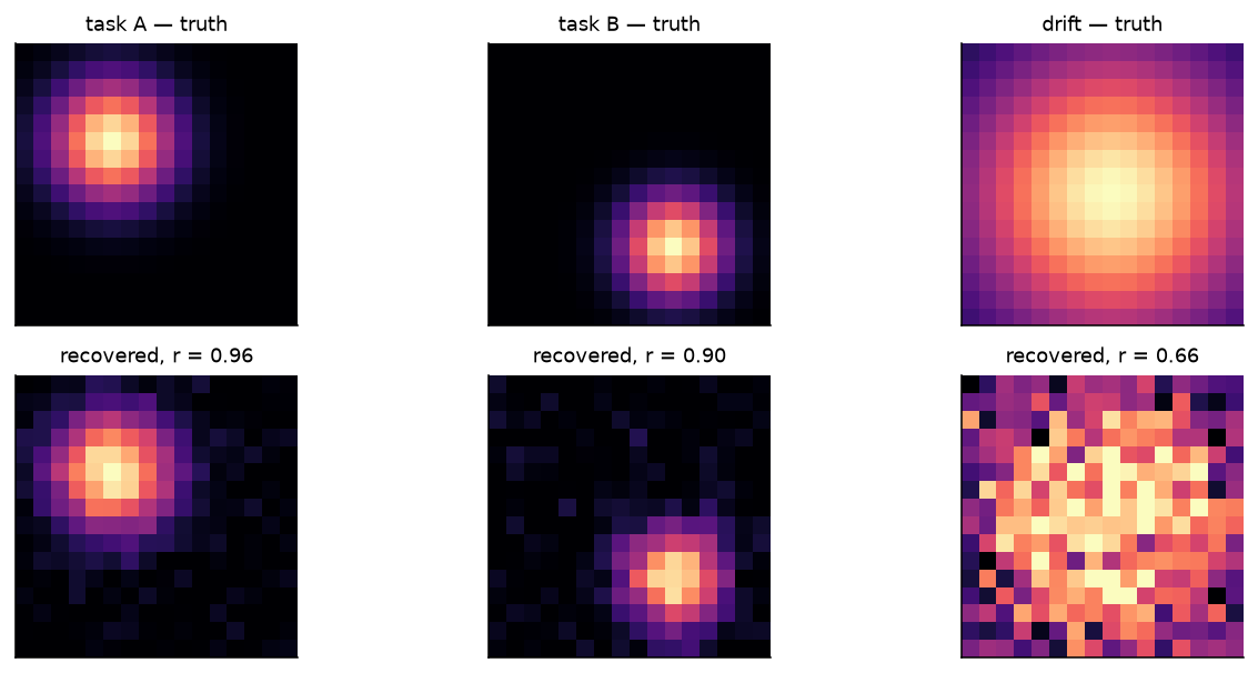

Figure 5: Recovered coefficient maps against the truth, one slice through each blob. The two task maps come back cleanly. The drift map does not, because its regressor is a slow ramp that noise can imitate.

8 Urban demand: a separable precision

Who does this. An urban data scientist putting an interval on a forecast over a week \(\times\) area \(\times\) offence-type array.

flowchart LR
  Y["<b>𝒴</b><br/>52 × 24 × 8<br/>weekly counts"] --> F["flatten to 192-vectors"]
  Y --> S["keep the modes"]
  F --> DC["dense Σ<br/>192 × 192<br/>rank 39 of 192"]
  S --> K["Σ<sub>area</sub> ⊗ Σ<sub>type</sub><br/>flip-flop MLE"]
  DC --> R1["singular — needs a ridge"]
  K --> R2["336 free parameters"]

Figure 6: One dense covariance over the flattened array, or one covariance per mode. Forty weeks are enough to fit the second. They are not enough to fit the first.

This is the one row of the table that is not an algebraic tensor inverse. Assuming that the covariance splits as \(\Sigma_{\text{area}} \otimes \Sigma_{\text{type}}\) is a claim you make about the world. The array does not tell you it is true.

It appears here for two reasons. People often call it “the tensor inverse” of a covariance, and it is not one. And on this data it does not pay off.

Code

counts, cmeta = D.chicago_counts()
Y = np.sqrt(counts.astype(float))  # variance-stabilise Poisson-like counts
train, test = Y[:40], Y[40:]
centre = train.mean(axis=0)
Ztr, Zte = train - centre, test - centre
dim = Ztr[0].size

print(f"{cmeta['n_incidents']:,} incidents, {cmeta['year']}, community areas 1-{max(cmeta['areas'])}")
print(f"array {counts.shape} -> {len(train)} training weeks, {len(test)} held out")
print(f"one week flattened is a {dim}-vector; the dense sample covariance has rank "
      f"{np.linalg.matrix_rank(Ztr.reshape(len(Ztr), -1).T @ Ztr.reshape(len(Ztr), -1))} of {dim}")

70,182 incidents, 2023, community areas 1-24
array (52, 24, 8) -> 40 training weeks, 12 held out
one week flattened is a 192-vector; the dense sample covariance has rank 39 of 192

Forty readings of a 192-dimensional vector cannot give a full-rank covariance. This is not bad luck with a small sample. It is arithmetic: 40 numbers cannot pin down 18,528.

The separable model fits one covariance per mode, using Dutilleul’s flip-flop algorithm. Whiten every other mode, take the sample covariance of the mode you are updating, then repeat until it settles.

Code

covs = D.flip_flop(Ztr, iters=60)
logdet = D.separable_logdet(covs)
quad = D.separable_quadform(Zte, covs)
sep_ll = float(np.mean(-0.5 * (dim * np.log(2 * np.pi) + logdet + quad)))
sep_params = sum(c.shape[0] * (c.shape[0] + 1) // 2 for c in covs)

Xtr, Xte = Ztr.reshape(len(Ztr), -1), Zte.reshape(len(Zte), -1)
S = Xtr.T @ Xtr / len(Xtr)
best_ll, best_ridge = -np.inf, None
for r in np.logspace(-4, 2, 25):
    Sr = S + r * np.trace(S) / dim * np.eye(dim)
    _, ld = np.linalg.slogdet(Sr)
    q = np.einsum("nd,de,ne->n", Xte, np.linalg.inv(Sr), Xte)
    ll = float(np.mean(-0.5 * (dim * np.log(2 * np.pi) + ld + q)))
    if ll > best_ll:
        best_ll, best_ridge = ll, r

# Where does the gain come from? Keep the mode variances, drop the mode
# correlations; then drop the variances too.
def sep_loglik(cs):
    q = D.separable_quadform(Zte, cs)
    return float(np.mean(-0.5 * (dim * np.log(2 * np.pi) + D.separable_logdet(cs) + q)))


diag_ll = sep_loglik([np.diag(np.diag(c)) for c in covs])
iso = [np.eye(d) for d in Ztr.shape[1:]]
iso[0] = np.eye(Ztr.shape[1]) * (Ztr**2).mean()
iso_ll = sep_loglik(iso)

print(f"{'model':<32} {'held-out log-lik':>17} {'free params':>12}")
print("-" * 63)
print(f"{'separable, area x type':<32} {sep_ll:17.1f} {sep_params:12,}")
print(f"{'separable, variances only':<32} {diag_ll:17.1f} "
      f"{sum(c.shape[0] for c in covs):12,}")
print(f"{'one variance for everything':<32} {iso_ll:17.1f} {1:12,}")
print(f"{'dense 192x192 + best ridge':<32} {best_ll:17.1f} {dim * (dim + 1) // 2:12,}")
print(f"\nthe dense model's ridge ({best_ridge:.2g}) was chosen on the held-out weeks themselves")

model                             held-out log-lik  free params
---------------------------------------------------------------
separable, area x type                      -192.7          336
separable, variances only                   -191.2           32
one variance for everything                 -192.7            1
dense 192x192 + best ridge                  -202.2       18,528

the dense model's ridge (1) was chosen on the held-out weeks themselves

The separable model beats the ridged dense one, and it uses 55 times fewer parameters. The dense model was even allowed to choose its ridge using the test weeks, which no honest pipeline would permit.

But the margin is small: about nine nats per week. A nat is a unit of log-likelihood, so nine nats is a modest gain, not a large one.

Now look at the third row. One single variance for the whole array scores as well as the separable model. On this data, the mode structure is not worth the extra work.

The fitted correlations reach only about 0.3 between community areas and about 0.1 between offence types. Once the weekly means are removed, very little is left for a covariance to explain.

One modelling choice drives that result, and it should be stated. The numbers above subtract a separate weekly mean for each area and each offence type.

Subtract a single overall mean instead. The area and type effects then stay inside the covariance, the fitted correlations climb past 0.85, and the mode structure starts to look impressive. But the ridged dense model then wins instead. The covariance is now describing a mean, and the Kronecker assumption is the wrong shape for a mean.

Neither way of centring makes this array a good example of separable covariance.

So this row of the table delivers less than it usually promises. As a statistical argument it is weak here. What remains is that the structured model can be fitted at all, and at full size that alone decides the question.

Code

full = counts.size
print(f"full array flattened: {full:,}-vector")
print(f"  dense covariance:   {full * (full + 1) // 2:,} free parameters, {full * full * 8 / 1e9:.1f} GB")
print(f"  separable, 3 modes: "
      f"{sum(d * (d + 1) // 2 for d in counts.shape):,} free parameters, "
      f"{sum(d * d for d in counts.shape) * 8 / 1e3:.1f} kB")
print(f"  and you have exactly 1 observation of that {full:,}-vector")

full array flattened: 9,984-vector
  dense covariance:   49,845,120 free parameters, 0.8 GB
  separable, 3 modes: 1,714 free parameters, 26.8 kB
  and you have exactly 1 observation of that 9,984-vector

Code

def to_corr(cov):
    d = np.sqrt(np.diag(cov))
    R = cov / np.outer(d, d)
    np.fill_diagonal(R, np.nan)
    return R


labels = [t.title().replace(" ", "\n") for t in cmeta["types"]]
fig, axes = plt.subplots(1, 4, figsize=(12.5, 3.9), width_ratios=[1.15, 1, 1.05, 0.8])
cmap = plt.get_cmap("RdBu_r").copy()
cmap.set_bad("#E9EBEF")

im = axes[0].imshow(to_corr(covs[0]), cmap=cmap, vmin=-0.3, vmax=0.3)
axes[0].set_title("community area correlation")
axes[0].set_xticks(range(0, 24, 4), range(1, 25, 4))
axes[0].set_yticks(range(0, 24, 4), range(1, 25, 4))

axes[1].imshow(to_corr(covs[1]), cmap=cmap, vmin=-0.3, vmax=0.3)
axes[1].set_title("offence-type correlation")
axes[1].set_xticks(range(8), labels, fontsize=6, rotation=90)
axes[1].set_yticks(range(8), labels, fontsize=6)
cbar = fig.colorbar(im, ax=axes[:2], shrink=0.82, pad=0.16,
                    label="correlation (diagonal masked)")
cbar.ax.yaxis.set_label_position("left")

sd_area = np.sqrt(np.diag(covs[0]))
sd_type = np.sqrt(np.diag(covs[1]))
axes[2].bar(np.arange(1, 25), sd_area / sd_area.mean(), color=PURPLE, width=0.75)
axes[2].set_title("scale per community area")
axes[2].set_xlabel("community area")
axes[2].set_ylabel("std dev / mean")
axes[2].axhline(1.0, color=INK, lw=0.8, ls="--")
axes[3].bar(np.arange(8), sd_type / sd_type.mean(), color=TEAL, width=0.7)
axes[3].set_title("scale per offence type")
axes[3].set_xticks(range(8), labels, fontsize=6, rotation=90)
axes[3].axhline(1.0, color=INK, lw=0.8, ls="--")
plt.show()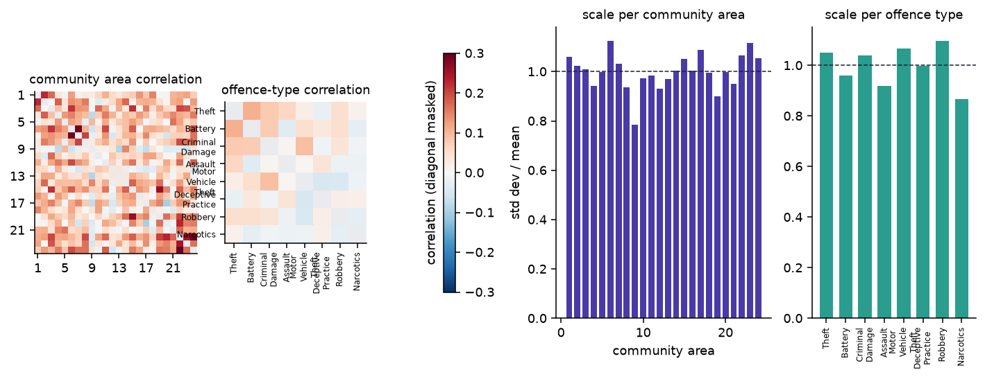

Figure 7: What the separable model actually found, which is not much. Left two panels: the fitted mode correlations with the diagonal hidden, on a ±0.3 scale. Right two: the scale of each area and each offence type, all within about 20% of one another. The structure is real but too weak to pay for itself, which is why one variance for the whole array scores as well.

9 Why not just flatten

Every number below was computed by a cell above.

Problem	Product	Inverse used	Operator, as a tensor	Operator, flattened	What flattening costs
Compliance	Einstein \(\circledast\)	multilinear Moore–Penrose	81 entries	\(9\times9\), rank 6	Nothing. Voigt drops exactly the null space. But converting back needs Reuter’s factors, and skipping them gives a 316% error off-axis
Hyperspectral	t-product \(*\)	regularised t-solve	13.5 MB	1.4 GB block-circulant	relative error 0.125 against 0.038; spectral angle 3.12° against 1.79°
Task maps	mode-\(n\) \(\times_n\)	mode-\(n\) pseudoinverse	\(120\times4\) solve	\(491{,}520 \times 16{,}384\) design, 64 GB	nothing, statistically. The flattening is the same estimator written out 4,096 times
Urban demand	— (separable model)	one precision per mode	336 parameters	18,528 parameters, rank 39 of 192	at this size, almost nothing. 9 nats of held-out log-likelihood, and one single variance matches that. On the full three-mode array, 0.8 GB and 49.8M parameters from one reading

Two of these four rows say that flattening is fine. A third says it is fine at this size and impossible at full size. Only one row is a clear win for the tensor.

So the question is never “tensor or matrix”. The question is whether your chosen flattening keeps the structure that the operator actually has.

Compliance. The flattening loses nothing, because the directions it throws away are the ones the operator sends to zero. You risk a conversion error, not a loss of information.
Task maps. The flattened GLM gives identical estimates. It wastes memory, but it is not wrong.
Hyperspectral. The flattening drops the cross-band slices of the operator, so it solves a different problem. The error it cannot get below is the band mixing it threw away.
Urban demand. The flattening asks for more parameters than the data can support. At three modes it asks for 0.8 GB of them from a single reading. But on this array the structure buys a model you can fit, and almost no accuracy. Check a structural assumption against the data. Do not adopt one just because the array has three modes.

10 Open problems

Matrix inverses are settled textbook material. Tensor inverses are not.

The list is still growing. Over roughly the last decade, researchers have carried the classical family of generalized inverses across to tensors under the Einstein product. That includes the Moore–Penrose inverse (Sun et al. 2016), the Drazin inverse (Behera et al. 2020), and the core and core-EP inverses (Sahoo et al. 2020). Papers defining more of them keep appearing. Nobody has agreed on a standard set, the way \(A^{-1}\) and \(A^{\dagger}\) are standard for matrices.
The numerics are behind the algebra. We know when most of these inverses exist, and whether they are unique. We know much less about how the algorithms behave in floating point, or what they cost to run. For several of them there is no agreed condition number to quote.
There are few tools. TensorLy covers decompositions well. For the inverses, you mostly write your own code from the definition. That is what src/tinv.py in this post does.
Do not overstate this. For elasticity, the Einstein-product inverse has been settled engineering practice for decades, under a different name. What is still open is the general theory and its numerics, not every use shown above.

11 Next steps

t-product solvers. t-GMRES and tensor Golub–Kahan (El Guide et al. 2021) find \(\mathcal{X}\) without ever building \(\mathcal{A}^{-1}\). On a full \(610\times340\times103\) scene, that is the difference between a program that runs and one that does not.
Tucker- and TT-format inverses. Worth timing when the operator itself will not fit in memory. The inverse usually has a higher rank than the operator, so the question that matters is how much higher, on your own problem.
CP-based approximate inverses. These give a rough approximation, not an inverse. They are cheap, but nothing is guaranteed.
Where TensorLy stops. It gives you CP, Tucker, TT and t-SVD. For the inverses above, the definitions are short and numpy is enough. The four in src/tinv.py are about a dozen lines each.

Problems. Pick. Products. Inverses. Follow. Flattening. Sometimes. Works. Check. First.

12 References

Brazell, M., Li, N., Navasca, C., and Tamon, C. (2013). Solving multilinear systems via tensor inversion. SIAM Journal on Matrix Analysis and Applications 34(2), 542–570.
Behera, R., Nandi, A. K., and Sahoo, J. K. (2020). Further results on the Drazin inverse of even-order tensors. Numerical Linear Algebra with Applications 27(5), e2317.
Dutilleul, P. (1999). The MLE algorithm for the matrix normal distribution. Journal of Statistical Computation and Simulation 64(2), 105–123.
El Guide, M., El Ichi, A., Jbilou, K., and Sadaka, R. (2021). On tensor GMRES and Golub–Kahan methods via the t-product for color image processing. The Electronic Journal of Linear Algebra 37, 524–543.
Hoff, P. D. (2011). Separable covariance arrays via the Tucker product, with applications to multivariate relational data. Bayesian Analysis 6(2), 179–196.
Kilmer, M. E., and Martin, C. D. (2011). Factorization strategies for third-order tensors. Linear Algebra and its Applications 435(3), 641–658.
Kolda, T. G., and Bader, B. W. (2009). Tensor decompositions and applications. SIAM Review 51(3), 455–500.
Kossaifi, J., Panagakis, Y., Anandkumar, A., and Pantic, M. (2019). TensorLy: tensor learning in Python. JMLR 20(26), 1–6.
Sahoo, J. K., Behera, R., Stanimirović, P. S., Katsikis, V. N., and Ma, H. (2020). Core and core-EP inverses of tensors. Computational and Applied Mathematics 39, 9.
Sun, L., Zheng, B., Bu, C., and Wei, Y. (2016). Moore–Penrose inverse of tensors via Einstein product. Linear and Multilinear Algebra 64(4), 686–698.
Hyperspectral Remote Sensing Scenes — Pavia University, ROSIS sensor; scenes provided by P. Gamba (University of Pavia), collection assembled by M. Graña, M. A. Veganzones and B. Ayerdi (UPV/EHU). Fetched here from an ungated mirror.
Crimes — 2001 to Present — City of Chicago open data portal.
Tensor Factorizations and Tensor Inverses — CP, Tucker, TT, t-SVD, and the four inverses on a synthetic cube.
Uses of Tensor Factorizations — the compression case.