Topological Data Analysis: Finding Clusters, Loops, and Voids Across Scales

Topological Data Analysis: Finding Clusters, Loops, and Voids Across Scales

Thanks to Andrei — a friend — and some of his math colleagues, whose discussion with me in Bogotá got me thinking about clustering vs. topology in the first place.

Introduction

Most clustering algorithms force you to commit to a single scale before you’ve even looked at the data. K-means needs k. DBSCAN needs eps. Hierarchical clustering needs a height at which to cut the dendrogram. Pick the wrong scale and a real multi-cluster structure collapses into one blob, or one meaningful group gets shredded into noise.

Topological Data Analysis (TDA) sidesteps this by not picking a scale at all. Instead of asking “what does the data look like at distance threshold \(\varepsilon\)?”, it asks “what does the data look like at every \(\varepsilon\) simultaneously, and which shapes survive across a wide range of them?” The shapes that survive — persist — are treated as signal. The shapes that flicker in and out of existence are treated as noise.

This post builds the idea up from scratch: simplices, the Vietoris-Rips filtration, and homology computed by hand on a 4-point example, before getting to the standard ripser/persim tooling and using persistence as a feature extractor for downstream ML.

Building Blocks: Simplices and the Vietoris-Rips Complex

A simplicial complex is just a generalization of a graph that’s allowed to have filled-in faces, not only vertices and edges:

• a 0-simplex is a point,
• a 1-simplex is an edge (2 points),
• a 2-simplex is a filled triangle (3 points),
• a 3-simplex is a filled tetrahedron (4 points), and so on.

Given a point cloud \(X = \{x_1, \dots, x_n\}\) and a radius \(\varepsilon \geq 0\), the Vietoris-Rips complex \(R_\varepsilon(X)\) is the simplicial complex built by a single rule:

\[ \{x_{i_0}, \dots, x_{i_k}\} \in R_\varepsilon(X) \iff \|x_{i_p} - x_{i_q}\| \leq \varepsilon \text{ for every pair } p, q. \]

In words: include a simplex whenever every pair of its vertices is within \(\varepsilon\) of each other. This is convenient because it’s determined entirely by the pairwise distance matrix — you never have to reason about higher-dimensional geometry directly, just check pairwise distances.

As \(\varepsilon\) grows from \(0\) to \(\infty\), more pairs satisfy the distance bound, so \(R_\varepsilon(X)\) only ever gains simplices: \(R_0(X) \subseteq R_{\varepsilon_1}(X) \subseteq R_{\varepsilon_2}(X) \subseteq \dots\). This nested, growing sequence of complexes is the filtration — the single object that encodes the shape of the data at every scale at once.

A First-Principles Example: The Hollow Square

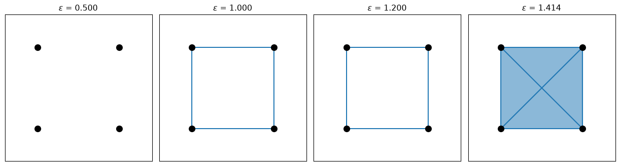
Four points at the corners of a unit square are enough to see everything: components merging, a loop opening, and that same loop closing back up.

import numpy as np
import matplotlib.pyplot as plt
from itertools import combinations

square = np.array([[0.0, 0.0], [1.0, 0.0], [1.0, 1.0], [0.0, 1.0]])
side, diagonal = 1.0, np.sqrt(2)


def plot_rips(points, eps, ax):
    n = len(points)
    dists = np.linalg.norm(points[:, None] - points[None, :], axis=-1)
    for i, j, k in combinations(range(n), 3):
        if dists[i, j] <= eps and dists[j, k] <= eps and dists[i, k] <= eps:
            ax.add_patch(plt.Polygon(points[[i, j, k]], alpha=0.3, color="tab:blue", zorder=1))
    for i, j in combinations(range(n), 2):
        if dists[i, j] <= eps:
            ax.plot(*zip(points[i], points[j]), color="tab:blue", zorder=2)
    ax.scatter(points[:, 0], points[:, 1], s=80, zorder=3, color="black")
    ax.set_title(f"$\\varepsilon$ = {eps:.3f}")
    ax.set_xlim(-0.4, 1.4)
    ax.set_ylim(-0.4, 1.4)
    ax.set_aspect("equal")
    ax.set_xticks([])
    ax.set_yticks([])


fig, axes = plt.subplots(1, 4, figsize=(13, 3.5))
for ax, eps in zip(axes, [0.5, side, 1.2, diagonal]):
    plot_rips(square, eps, ax)
plt.tight_layout()
plt.show()

Reading left to right: at \(\varepsilon = 0.5\) nothing is close enough to connect — 4 separate points. At \(\varepsilon = 1\) (the side length) the 4 boundary edges appear and the points become one connected ring — but the diagonals (\(\sqrt{2} \approx 1.414\)) are still too far apart to connect, so the square stays hollow: a genuine loop has opened up. At \(\varepsilon = 1.2\) nothing has changed yet — the loop persists. Only at \(\varepsilon = \sqrt{2}\) do the diagonals connect, triangles fill in, and the loop closes.

From boundaries to Betti numbers, computed directly

This is the payoff of the first-principles approach: homology is genuinely just linear algebra on the simplices, and we can compute it ourselves without a library. A \(k\)-chain is a formal sum of \(k\)-simplices; the boundary map \(\partial_k\) sends a \(k\)-simplex to the alternating sum of its \((k-1)\)-dimensional faces. A cycle is a chain with zero boundary (\(\ker \partial_k\)); a boundary is a chain that is itself the boundary of something one dimension up (\(\operatorname{im} \partial_{k+1}\)). The \(k\)-th Betti number counts cycles that aren’t boundaries:

\[ \beta_k = \dim \ker \partial_k - \dim \operatorname{im} \partial_{k+1}. \]

def rips_simplices(points, eps, max_dim):
    n = len(points)
    dists = np.linalg.norm(points[:, None] - points[None, :], axis=-1)
    simplices = {0: [(i,) for i in range(n)]}
    for dim in range(1, max_dim + 1):
        simplices[dim] = [
            combo
            for combo in combinations(range(n), dim + 1)
            if all(dists[i, j] <= eps for i, j in combinations(combo, 2))
        ]
    return simplices


def boundary_matrix(simplices_k, simplices_km1):
    index = {s: i for i, s in enumerate(simplices_km1)}
    d = np.zeros((len(simplices_km1), len(simplices_k)))
    for col, simplex in enumerate(simplices_k):
        for i in range(len(simplex)):
            face = simplex[:i] + simplex[i + 1 :]  # drop vertex i -> a face
            d[index[face], col] = (-1) ** i
    return d


def betti_numbers(points, eps, max_dim=2):
    simplices = rips_simplices(points, eps, max_dim)
    ranks = {0: 0}
    for dim in range(1, max_dim + 1):
        if simplices[dim] and simplices[dim - 1]:
            ranks[dim] = np.linalg.matrix_rank(boundary_matrix(simplices[dim], simplices[dim - 1]))
        else:
            ranks[dim] = 0
    betti = {}
    for dim in range(max_dim):
        cycles = len(simplices[dim]) - ranks[dim]      # dim ker(d_dim)
        boundaries = ranks.get(dim + 1, 0)              # dim im(d_{dim+1})
        betti[dim] = cycles - boundaries
    return betti


for eps in [0.5, side, 1.2, diagonal]:
    print(f"eps = {eps:.3f}:  betti_0 = {betti_numbers(square, eps)[0]},  betti_1 = {betti_numbers(square, eps)[1]}")

eps = 0.500:  betti_0 = 4,  betti_1 = 0
eps = 1.000:  betti_0 = 1,  betti_1 = 1
eps = 1.200:  betti_0 = 1,  betti_1 = 1
eps = 1.414:  betti_0 = 1,  betti_1 = 0

That matches the pictures exactly: \(\beta_0\) drops from 4 to 1 once the ring connects at \(\varepsilon = 1\); \(\beta_1\) turns on at the same moment (a loop is born) and switches back off at \(\varepsilon = \sqrt{2}\) (the loop dies, filled in by the two triangles). Cross-checking against ripser confirms it:

from ripser import ripser

dgms = ripser(square, maxdim=1)["dgms"]
print("H0 (birth, death):\n", dgms[0])
print("H1 (birth, death):\n", dgms[1])

H0 (birth, death):
 [[ 0.  1.]
 [ 0.  1.]
 [ 0.  1.]
 [ 0. inf]]
H1 (birth, death):
 [[1.         1.41421354]]

The single \(H_1\) row should read [1.0, 1.41421356] — born at \(\varepsilon = 1\), dies at \(\varepsilon = \sqrt{2}\), exactly as read off the plot.

Persistent Homology as “Clustering, Expanded Across Dimensions”

Look again at how \(\beta_0\) was computed above: \(\dim \ker \partial_1\) counts vertices, \(\operatorname{im}\partial_1\)’s rank tells you how many independent edges it took to connect them, and the difference is the number of connected components. That is exactly what single-linkage clustering computes: threshold a distance graph at \(\varepsilon\) and count connected components. \(H_0\) isn’t analogous to clustering — it is clustering, expressed in the language of boundary maps.

Now notice that \(\beta_1\) is computed by the identical operation, just one dimension up: instead of 0-chains (points) modulo boundaries of 1-chains (edges), it’s 1-chains (loops) modulo boundaries of 2-chains (filled patches). Two loops get treated as “the same” if their difference bounds a filled-in disk — which is precisely the loop version of “two points get treated as the same cluster if they’re connected by a path.”

So the general pattern is:

\[ \beta_k = \underbrace{\text{(all $k$-dimensional cycles)}}_{\text{the ``things''}} \Big/ \underbrace{\text{(the ones that bound a $(k{+}1)$-dimensional patch)}}_{\text{``trivial'' cycles}} \]

• \(k=0\): points modulo paths \(\to\) clusters.
• \(k=1\): loops modulo filled disks \(\to\) independent holes/handles.
• \(k=2\): enclosed shells modulo filled solids \(\to\) voids.

Clustering is the \(k=0\) special case of one general machine. Persistent homology runs that same machine at every dimension \(k\) and every scale \(\varepsilon\) at once, which is the sense in which TDA is clustering expanded across both dimension and scale simultaneously — not a metaphor, but the same boundary/quotient computation applied more generally.

Loops and Voids on Real(ish) Data

The hollow square is one loop by hand. Here’s the same idea on a noisy point cloud, using ripser/persim instead of the from-scratch code above.

from sklearn.datasets import make_circles, make_blobs
from persim import plot_diagrams

rng = np.random.default_rng(42)

ring, _ = make_circles(n_samples=200, noise=0.05, factor=0.6, random_state=42)
blobs, _ = make_blobs(n_samples=200, centers=3, cluster_std=0.4, random_state=42)

fig, axes = plt.subplots(2, 2, figsize=(10, 8))

for ax, data, title in zip(axes[0], [ring, blobs], ["Noisy ring", "Three blobs"]):
    ax.scatter(data[:, 0], data[:, 1], s=10)
    ax.set_title(title)
    ax.set_aspect("equal")

for ax, data, title in zip(
    axes[1], [ring, blobs], ["Ring: persistence diagram", "Blobs: persistence diagram"]
):
    dgms = ripser(data, maxdim=1)["dgms"]
    plot_diagrams(dgms, ax=ax, show=False)
    ax.set_title(title)

plt.tight_layout()
plt.show()

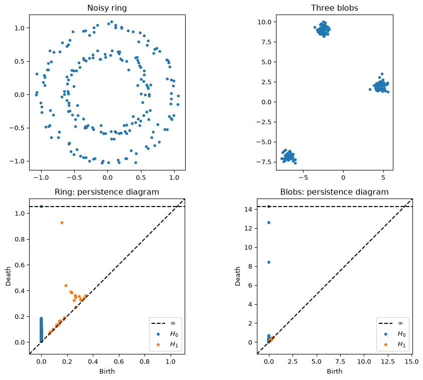
For the ring, one \(H_1\) (orange) point sits far above the diagonal — the loop around the ring, persisting from roughly the point-spacing scale up to the ring’s diameter. K-means or DBSCAN would either carve this ring into arbitrary chunks or lump it into one blob; neither captures “it’s a ring.” For the three blobs, \(H_1\) hugs the diagonal (no real loops), while \(H_0\) shows three long-lived components before they merge into one — “three clusters,” read straight off the diagram without ever choosing \(k\).

Verifying \(H_0\) persistence = single-linkage clustering, on real data

from scipy.cluster.hierarchy import linkage

dgm0 = ripser(blobs, maxdim=0)["dgms"][0]
death_times = np.sort(dgm0[np.isfinite(dgm0[:, 1]), 1])

Z = linkage(blobs, method="single")
merge_heights = np.sort(Z[:, 2])

print("H0 death times match single-linkage merge heights:", np.allclose(death_times, merge_heights))

H0 death times match single-linkage merge heights: True

How TDA Differs From Traditional Clustering

Aspect	Traditional clustering (k-means, DBSCAN, GMM)	Topological data analysis
Scale	One fixed scale, set by a hyperparameter (k, eps, n_components)	All scales at once, encoded in a filtration
Output	A single partition of points	A persistence diagram: every topological feature, born and dying across all scales
Shape assumptions	Often assumes convex/globular clusters (k-means) or one global density (DBSCAN)	None — captures components, loops, voids, and higher-dimensional structure
Noise vs. signal	No built-in separation; depends entirely on hyperparameter choice	Persistence is the noise filter: short lifetime = noise, long lifetime = structure
Sensitivity	Different k/eps can give qualitatively different answers	Deterministic given a distance and filtration; the diagram is stable under small perturbations of the data
Cost	\(O(n)\)–\(O(n^2)\) depending on algorithm	\(O(n^3)\) or worse for full Rips persistence; needs subsampling/landmarks at scale

The practical upshot: clustering answers “what is the grouping?” for a scale you had to guess in advance. TDA answers “at which scales, and how confidently, does structure exist?” — and it can describe loops and voids that no partition of points into disjoint clusters could ever represent.

TDA as a Feature Extractor for Downstream ML

Persistence diagrams are useful on their own, but they’re also a genuinely different way to featurize data for standard supervised learning. A diagram is a multiset of points, which isn’t directly usable by most ML models — so it gets vectorized into a fixed-length summary. Common approaches:

• Summary statistics: max lifetime, total lifetime (sum of all persistences), count of features above a persistence threshold, persistence entropy.
• Persistence images: rasterize the diagram (after rotating birth/death into birth/lifetime coordinates) into a fixed-size grid, weighted by persistence — now it’s an image you can feed to a CNN or any tabular model.
• Persistence landscapes: a functional summary that lives in a vector space, so you can average diagrams, compute distances, and use them in kernel methods.

This is genuinely used in practice — classifying time series via Takens’ delay embedding + persistence, characterizing material microstructures, distinguishing molecular conformations — anywhere “shape” is informative but hard to hand-engineer.

Toy example: classifying point-cloud shape from persistence features

from sklearn.ensemble import RandomForestClassifier
from sklearn.model_selection import train_test_split


def sample_blob(n, rng):
    return rng.normal(size=(n, 2))


def sample_ring(n, rng, radius=1.0, noise=0.05):
    theta = rng.uniform(0, 2 * np.pi, n)
    r = radius + rng.normal(0, noise, n)
    return np.column_stack([r * np.cos(theta), r * np.sin(theta)])


def persistence_features(point_cloud):
    """Vectorize a point cloud's H1 persistence diagram into 3 summary numbers."""
    h1 = ripser(point_cloud, maxdim=1)["dgms"][1]
    if len(h1) == 0:
        return np.zeros(3)
    lifetimes = h1[:, 1] - h1[:, 0]
    return np.array([lifetimes.max(), lifetimes.sum(), (lifetimes > 0.1).sum()])


rng = np.random.default_rng(0)
X, y = [], []
for _ in range(60):
    X.append(persistence_features(sample_blob(100, rng)))
    y.append(0)  # "blob" shape class
    X.append(persistence_features(sample_ring(100, rng)))
    y.append(1)  # "ring" shape class

X, y = np.array(X), np.array(y)
X_train, X_test, y_train, y_test = train_test_split(X, y, test_size=0.3, random_state=0)

clf = RandomForestClassifier(n_estimators=100, random_state=0)
clf.fit(X_train, y_train)
print(f"Test accuracy: {clf.score(X_test, y_test):.2f}")

Test accuracy: 1.00

Three numbers derived from persistent homology — max loop lifetime, total loop lifetime, count of significant loops — are enough to separate “blob-shaped” from “ring-shaped” point clouds. No pixel grid, no distance-to-centroid feature engineering: the topology itself is the feature.

Practical Considerations

• Cost. Computing full Rips persistence is roughly \(O(n^3)\) in the worst case. For anything beyond a few thousand points, subsample, use landmark/witness complexes, or cap the maximum simplex dimension you compute.
• Distance choice still matters. TDA removes the scale hyperparameter, not the metric one — Euclidean vs. cosine vs. a learned distance still changes which shapes you find.
• It complements clustering, not replaces it. A common pattern: use \(H_0\) persistence to get a principled, noise-aware read on how many clusters exist and how confident to be in each merge, then run k-means or DBSCAN with that scale as an informed choice rather than a guess.
• Related but distinct: Mapper. The Mapper algorithm (cover the data, cluster within each cover element, connect overlapping clusters into a graph) produces a different kind of multi-scale summary — a compressed graph rather than a persistence diagram — and is worth a separate post.
• Libraries. ripser/persim (used above) are lightweight and fast for Rips persistence in low dimensions; GUDHI and giotto-tda cover a broader set of complexes, vectorizations, and scikit-learn-compatible transformers.

Key Takeaways

• TDA studies data across every scale at once via a filtration, instead of committing to one scale up front like k-means or DBSCAN.
• Homology is computable directly from a boundary-map matrix’s rank and nullity — \(\beta_k = \dim\ker\partial_k - \dim\operatorname{im}\partial_{k+1}\) — no black box required.
• \(\beta_0\) persistence is exactly single-linkage hierarchical clustering; \(\beta_1, \beta_2, \dots\) apply the identical cycles-modulo-boundaries computation one dimension up, which is the precise sense in which TDA is clustering expanded across dimensions.
• Persistence — how long a topological feature survives across the filtration — is a principled, built-in way to separate real structure from sampling noise.
• Vectorized persistence diagrams (summary stats, persistence images, landscapes) are a legitimate, general-purpose feature extractor for downstream supervised ML.

Questions for Reflection

1. If \(\beta_0\) persistence recovers single-linkage clustering, what would a “persistence-aware” version of k-means or DBSCAN look like?
2. For a dataset where you do know the right number of clusters in advance, does TDA still add value — or is it strictly a discovery tool?
3. How would you choose a persistence threshold to separate “signal” from “noise” without just reintroducing a hidden hyperparameter?