Variational AutoEncoders

Part 1

KAHOOT.IT

Objective

• Understand generative AI from VAE model families
• Try some applications
• Use Keras, PyTorch, JAX API
• References
• Kingma & Welling (2019)

Motivation

• Why?
• How is the natural environment?
• What has this do with genetics?

Generative AI

• Discriminative

f: (x, y)→ t

f(y) discriminative learning [notation: f(y) = f_x(y) = f(y;x) = f(y|x) ], f characterizes p(y | x)

• Generative

g: x→?(x)

g(x) generative learning, g characterizes p(x)

p: Ω→[0, 1]

probability density

s: [0, 1]→Ω

simulator

• Often:
  • f models p
  • g models p or s
• s(x) is Generative AI (ChatGPT, Gemini, Claude, Stable Diffusion)
• Generative AI outputs transformations of random numbers
• transformations learned from data

Outline

• Encoder & Decoder = AutoEncoder
• Compression & Decompression Analogy
• AutoEncoder
• Example in Keras & PyTorch & JAX
• Jensen’s Inequality, Variational Bayes & VAE Derivation
• Variational AutoEncoder
• Compression & Decompression Analogy
• Example in Keras & PyTorch & JAX

Compression & Decompression: Reality

• Lossless Compression:
  • count frequencies, replace with shorter code:
    • RLE
    • Huffman
    • Lempel-Ziv (used for png, gzip, etc)
• Lossy Compression:
  • Reduce data, but permit errors
    • FFT (jpeg, h.264, mp3)
      • filter out low frequencies (high variance neighbourhoods)
      • keep low frequencies (low variance neighbourhoods)
    • local regression (WebP)
    • New ideas with neural compression are starting to emerge (not current VAEs)

Encoder & Decoder = AutoEncoder

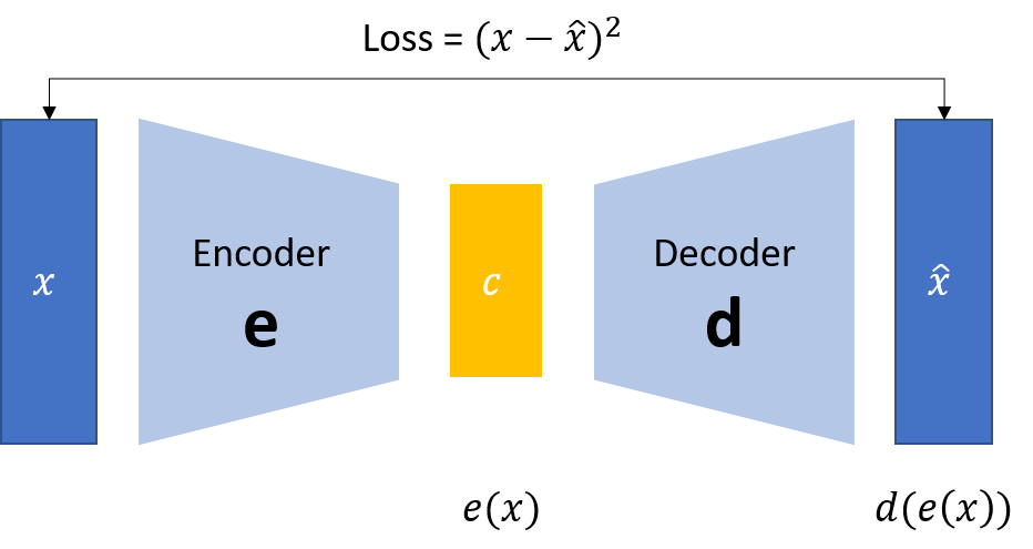
AutoEncoder

• Observe X ⊆ Ω, X:data observed, Ω: All possible data

encoder

e: X ↦ Z

decoder

d: Z ↦ X

• e & d are relatively well behaved locally (mostly)

reconstructor: r = (d ∘ e)

r: X ↦ Z ↦ X

d & e are neural networks; at perfection

e ≐ inverse(d)

can measure reconstruction loss

L: (Ω , r) ↦ ℝ≥0

g = (d ∘ s)

g: [0, 1] ↦ Z ↦ Ω

• g produces random variates that are synthetics of X, or generative AI

Compression & Decompression

• e is compression of data from X to Z space
• d is decompression of data from Z to S space
• This composition is sometimes called the bottleneck architecture

Compression

Decompression

PCA & Linear AutoEncoder

• Linear AutoEncoder
  • encoder: linear projection of X
    • some space Z
    • projection columns
      • no restrictions
  • learn by gradient descent
    • over reconstruction loss

• PCA
  • principal components: linear projection of X
    • some space Z
    • projection columns
      • restrictions
        • must be orthogonal
        • components ordered by variance
  • learn by eigen decomposition (via SVD)
    • over covariance(X)

Example: NumPy, Keras & PyTorch

• autoencoders notebook

Variational Compression & Decompression

Variational AutoEncoders

• same e & d
• change compressed space
  • make similar data points in sample space cluster
  • new loss = reconstruction loss + regularizer
    • regularizer
  • Kullback-Leibler divergence

Variational AutoEncoders: Mathematics

• convex function
• weighted sum of convex function
  • Evaluated at different points:
    • Still a convex function
• use 2 to prove Jensen’s inequality
• use 3 to prove ELBO inequality
  • expansion of p(x):
    • as an integral over some latent space z
    • multiply and divide by 1
    • replace 1 by q(z)/q(z), for any prob distribution q
    • bound p(x) by ELBO
• set q = MVN(𝝻, 𝞂)
• fascinating tricks (reparameterization, known identities)
• learn weights of encoder, decoder & parameters of MVN(𝝻, 𝞂) using SGD

Example: Keras

• Keras 3.0 VAE

Example: PyTorch

• Repo of PyTorch-VAEs

Pros & Cons

Pros	Cons
Generates new, similar data	Blurry reconstructions
Structured latent space	Mode collapse
Regularization prevents overfitting	Inference complexity
Efficient for large datasets	Training can be unstable
Provides insights into data structure	Non-convex optimization landscape

Extensions

• Beta-VAE
  • weight KL regularizer with hyperparameters
• VQ-VAE
  • k-means in compressed space Z
• Conditional VAE
  • append label to Z space
• lnfoMax VAE:
  • KL + additional regularizer:
    • weight on mutual information measure

?s

?s

?s

Variational AutoEncoders

Part 2

Outline

• GenAI & AutoEncoder recap
• Keras API
• VAE maths
  • ELBO
• Generation of variants
  • MNIST
  • human_nontata_promoters
• PyTorch API

Generative AI

• Discriminative

f: x→y

f(y) discriminative learning [notation: f(x) = f_y(x) = f(y;x) = f(y|x) ]

• Generative

g: (x,y) →?(x,y)

g(x,y) generative learning [can replace (x,y) with just x, g: x → ?(x)]

p: Ω→[0,1]

explicit probability density

s: [0,1]→Ω

simulator making use of p (implicit probability density)

• Often:
  • f models p
  • g models p or s
• s(random_number) is Generative AI (ChatGPT, Gemini, Claude, Stable Diffusion)
• Generative AI outputs transformations of random numbers
• transformations learned from data

Exercise: Individual

• Give 4 examples of discriminative functions from well known models?
• Should discriminative functions always be probability functions?
• Give 4 examples of generative functions from well known models?
• Should generative functions always be probabilities?
• if you remap (x, y) to x, what does this mean for generative models?
• The other way — remap x → (x, y)
• Generative or Discriminative: next word prediction & LLM models?

Types

Model Type	Supervised	Unsupervised
Generative Explicit	Definition: Models that explicitly learn the joint distribution P(x, y).	Definition: Models that learn the data distribution without labels.
	– Naive Bayes	– Gaussian Mixture Models (GMM)
	– Conditional Random Fields (CRFs)	– Variational Autoencoders (VAEs)
	– Hidden Markov Models (HMMs)	– Latent Dirichlet Allocation (LDA)
Generative Implicit	Definition: Models that generate samples without explicitly modeling the joint distribution.	Definition: Models that create new data based on learned patterns without labels.
	– Conditional GANs (cGANs)	– GANs (Generative Adversarial Networks)
	– Supervised Diffusion Models	– Score-Based Generative Models
	– Supervised Neural Processes	– Normalizing Flows
Discriminative Models	Definition: Models that predict P(y | x), focusing on decision boundaries.
	– Logistic Regression	– k-Means Clustering
	– Support Vector Machines (SVMs)	– Principal Component Analysis (PCA)
	– Neural Networks for Classification/Regression	– Hierarchical Clustering

PCA & Linear AutoEncoder

• Linear AutoEncoder
  • encoder: linear projection of X
    • some space Z
    • projection columns (learn weight matrix)
      • no restrictions
  • decoder: map Z→ X linearly (learn linear projection; weight matrix)
  • learn by gradient descent
    • over reconstruction loss

• PCA
  • encoder: linear projection of X
    • some space Z
    • projection columns (principal components)
      • restrictions
        • must be orthogonal
        • components ordered by variance
  • decoder: map Z → X linearly (transpose of ordered eigenvector matrix)
  • learn by eigen decomposition (via SVD)
    • over covariance(X)

Exercise: Group

• Split in 2 groups:
• Write out key function names, parameters, and dimensions of domain & co-domain for a linear autoencoder.
• BONUS:
• Write out the same for PCA. Try to keep to similar names & notation.
• colab notebook

DL Frameworks

Why Frameworks

• Accelerated hardware for data computations, needs special software

Feature	TPU	Nvidia H100	CPU
Core Count	Up to 256	16,896 CUDA Cores 640 Tensor Cores	4 to 64
Core Type	Specialized for ML	Specialized (CUDA and Tensor Cores)	General-purpose cores
Matrix Multiplication	Optimized for tensors with high throughput	Accelerated by Tensor Cores using mixed precision; handles 4x4 sub-matrices per clock cycle	Standard, less efficient without parallelism
LU Decomposition	Optimized for deep learning	Parallelized using CUDA; relies on optimized libraries (e.g., cuBLAS, cuSolver)	Sequential, less efficient
Memory Bandwidth	Very high	High (up to 900 GB/s with HBM3)	Moderate (25-100 GB/s)
Power Efficiency	Highly efficient for ML	Efficient but power-hungry	Less efficient for parallelism
Best Use Cases	Large-scale ML training	Deep learning, HPC, and graphics	General tasks, simple ML
CPU Needs	Minimal for ML workloads	Significant for mixed workloads	High for general computing

Keras: Progressive API Framework

• A high level DL API https://github.com/keras-team/keras/issues/13707
• Use abstractions (verbs) to hierarchically hide the details
• Keras 3.0: supported backend PyTorch, JAX, TF, R & MLX (soon)
• prototyping & engineering (YouTube, WayMo, Google, Microsoft, AWS)

Exercise: Keras APIs

• An API is a set of rules for software applications to communicate. Keras has 3 types:
• Sequential
• Model
• Functional
• Work in groups of 3. Understand the API, populate slides

Keras API Sequential

• Definición del Modelo: Inicializa el modelo secuencialmente para apilar capas en orden.
• Agregar Capas:
  • Se añaden capas como Dense, Conv2D, etc., en secuencia para formar la arquitectura.
  • Se puede definir una capa Input para especificar la forma de entrada, o dejar que el modelo la infiera en el primer uso.
• Compilación del Modelo: Define el optimizador y la función de pérdida.

   Entrada
      |
+----------+     +----------+     +----------+
|   Capa   | ->  |   Capa   | ->  |   Capa   |
|de entrada|     |  oculta  |     |de salida |
+----------+     +----------+     +----------+
      |                |                |
    Salida           Salida           Salida
  intermedia       intermedia          final

• Group 1: Sequential API

• Group 2: Model Class API
• Forma más flexible de crear una red neuronal mediante herencia directa de clases/modelos.
• Permite arquitecturas personalizadas

class MyModel(Model):
    def __init__(self):
        super(MyModel, self).__init__()
        self.dense1 = Dense(64, activation='relu')
        self.dense2 = Dense(32, activation='relu')
        self.output_layer = Dense(1, activation='sigmoid')

• Group 2: Model Class API
• Es ideal cuando necesitas construir redes neuronales personalizadas y complejas que no pueden realizarse con las APIs secuenciales o funcionales de Keras.

Functional API

• The Keras Functional API Es una forma de construir modelos en frameworks de aprendizaje profundo.
• Modelos complejos y personalizados, múltiples entradas y salidas, redes neuronales no lineales y arquitecturas sofisticadas
• Las capas se pueden conectar directamente, donde la salida de una capa se convierte en la entrada de la siguiente.
• Los modelos de la Functional API pueden aceptar múltiples entradas y producir múltiples salidas, lo que te permite definir tareas como la generación de descripciones de imágenes
• Puedes reutilizar capas en diferentes partes del modelo, lo que es útil en redes siamés y otros modelos con características compartidas.

Functional API

  Input1 (shape=(3,))    Input2 (shape=(3,))
          |                      |
       Dense(4)               Dense(4)
          |                      |
          |--- Branch 1    Branch 2 ---|
                     |        |
                     |        |
             Concatenate (combines outputs)
                          |
                  Dense(1) (output layer)
                          |
                    Final Output

Examples with non-sequential processing:

• ResNet
• Attention
• Transformers

KAHOOT.IT

VAEs: Mathematics Exercise

• convex function
• weighted sum of convex function
  • evaluated at different points:
    • still a convex function
• use 2 to prove Jensen’s inequality
• use 3 to prove ELBO inequality
  • expansion of p(x):
    • as an integral over some latent space z
• expansion of log(p(x))
  • multiply and divide by 1
    • replace 1 by q(z)/q(z), for any prob distribution q
  • bound log(p(x)) by ELBO
• set q = MVN(𝝻, 𝞂)
• tricks (reparameterization, known identities)
• substitute vae, decoder, encoder densities
• learn weights of encoder, decoder & parameters of MVN(𝝻, 𝞂) using SGD

Mathematical Insights

• Variational Inference
• VAE raises the bound on log evidence
• encoder is approximating posterior on Z | X
  • prior on Z is standard MVN
• decoder is generator of X | Z
• Mixed Effects Model
• Fixed: weights
• Random: latent variables
• VAE is mixed effects nonlinear model

Exercise: Generators

• Extract Generator from VAE
• MNIST, use this colaboratory notebook
• Now for the human_nontata_promoters dataset
• Hyperparameter tune (use optuna)
  • based on evaluation metrics (for gene sequences)
• Generate variates
• Compare output to AutoEncoder

KAHOOT.IT

Exercise: VAE

• Human nonTATA promoter toy dataset
• Train VAE to generate novel promoters
  • Use Keras to rework autoencoders notebook as a AE, and then VAE
• Hyperparameter tuning with Optuna
• EXTRA
• Do the same with PyTorch (no lightning)

PyTorch

• DL Framework
• Supported by PyTorch Foundation
• More low level than Keras
• Preferred by researchers
• Less performant than TensorFlow
• Closer to model mathematics
• Imperative style, dynamic computation graph

?s