Tensors for Machine Learning — from real data to modern models. Ravi Kalia and Sebastian Laverde Chunza.

Say this out loud: nobody is expected to know tensor theory. Every new term is defined the first time it appears. Students are ESL (Colombia) — speak slowly, avoid idiom, and name the Spanish cognates early: eje, descomposición, contracción, convolución.

Predict first: same numbers — still a voice?

Play the voice as built, then switch the layout and play it again: the same 263,169 numbers, only in a different order.

Open the voice widget ↗

Sound on — test the room’s speakers before people arrive; this only works if they can hear it. Press play on the voice as the transform built it: it sounds like a voice. Switch Layout to transposed and press play again: same 263,169 numbers, only reordered, and it is noise.

The one number to point at: 263,169 — say it out loud both times, so the room hears that nothing was lost.

Ask why a transpose that loses nothing still ruins the sound — and do not answer. Promise the room that section 04 and the wrap-up’s last slide both come back to this.

The workshop idea: four cards show scalar, vector, matrix and tensor as 0D, 1D, 2D and ND arrays, each defined by its shape. The guiding question of the day: before operating, what does each axis represent?

Four ideas, one object. The whole day in four cards. Card one: a tensor generalizes a matrix. A scalar has no axes, a vector one, a matrix two, and a tensor as many as the data needs. Card two: it holds the data. Images, video frames, taxi trips and prices are all one box of numbers, and every axis stands for something. Card three: its axes can be moved. Transpose permutes them. Reshape re-reads the same flat numbers, so the same shape can carry a different meaning. Card four: it factors. Numbers into primes, quadratics into roots, matrices into LU, QR and SVD, and tensors too. Where an inverse does not exist, the pseudoinverse answers. Carry this all day: before you operate on a tensor, name its axes.

This is the map of the day, and the only slide that shows all four ideas at once. Spend a minute on it, not five. Each card is opened properly later: card 1 in section 01, card 2 in sections 02 and 03, card 3 in section 04, and card 4 in sections 07, 09, 10 and 11.

The fourth card is the one to sell. Students already factor numbers and solve quadratics. The claim is that factorization is the same move each time, applied to a bigger object. That is the promise section 09 collects on.

Say “axes”, not “dimensions”, from here on — and remember the “rank” warning is due at the start of Part I.

Real data, real problems. Four real datasets used throughout the workshop: handwritten digits, stained histology, California housing, and NYC taxi trips. Each carries the role it plays later.

The point of the grid is that every card is a link: students can go and look at the source themselves, and several will. Name the two that surprise people — the digits are the UCI 8x8 set, not MNIST, and the cell is a phase image from a hologram rather than a stained slide — the histology card beside it is the stained one.

Image credits, none of them required: taxis Ferdinand Stohr, DC-3 Bernard Spragg, histopathology Mikael Haggstrom MD, tract housing Alfred Twu (Wikimedia Commons); storm Nicolas Vigier (Commons); voice Bart Massey — all CC0. Digits, cell, histology and waveform are rendered from the data itself by scripts/gen_thumbnails.py; those are CC0 too, except the histology, which skimage documents as having no known copyright restrictions.

Agenda — 210 minutes

Start Time	Duration (min)	Part	Segment Name
00:00	5	—	Setup and welcome
00:05	20	I	What a tensor is
00:25	20	II	Thinking in N dimensions
00:45	30	III	Indexing & broadcasting · Reshape & transpose
01:15	10	🎯	Kahoot 1 + break
01:25	15	III	Video pipeline design (group)
01:40	15	IV	Contraction with einsum
01:55	5	—	Break
02:00	15	IV	Inverses and the pseudoinverse
02:15	5	🎯	Kahoot 2
02:20	25	IV	Recursion · Matrix factorizations
02:45	5	—	Break
02:50	15	IV	Tucker decomposition
03:05	5	🎯	Kahoot 3
03:10	15	IV	Tensor factorizations
03:25	5	—	Wrap-up and take-homes

Give the “rank” warning at the start of Part I, not later. It is the single most reliable source of confusion in this workshop. Chapter 2 uses rank for the number of independent columns; tensor theory usually means the number of axes. Today, say “order” for the number of axes, and “rank” only in Chapter 2’s sense.

Rhythm, so the room knows what to expect: a section opens on a prediction, then an exercise with its own check, and most close on a group task of 6 to 8 minutes whose three-line share-back goes in Discord. The run sheet in the facilitator guide has every section’s split. Every section runs its notebook’s core route only; Explore later is for afterwards.

00 · Setup and welcome

—

5 min

Practise today

Name possible axes and predict a slice in the entry check.

Explore later

After the entry check, revisit data-quality examples. Complete runtime setup before class.

Colab ↗

Setup was pre-work. Collect the individual entry check before discussion.

01 · What a tensor is

I

20 min

Practise today

Name image axes and distinguish shape, order, and element count.

Explore later

Extract slices and fibers, and unfold images into matrices.

Colab ↗

📖 NumPy to JAX ↗

Open on the photo: how many numbers hold it? 512 × 512 × 3 = 786,432. The slot is 4 minutes modelling one shape and 16 for Exercise 1 with a partner check; the three computing slides after the two images are a skim, not a lesson. Listen for “rank” meaning the number of axes, and say “order”.

Map of factorizations: six matrix and tensor factorizations arranged on a ladder from LU through Cholesky, QR, SVD, Tucker and CP, each with one phrase describing what it buys.

Section 09 walks this map on real data: every factorization written as a constrained optimization, the cost of each one derived and then measured, and SVD as the best rank-k approximation there is. The “which one, and what does it cost me” question this ladder raises is answered two hours later, in the room.

📖 Why so many matrix factorizations? ↗

Prime factorization is unique up to ordering — the cleanest case on the slide. Generic low-rank matrix factors have gauge freedom (the \(M\)/\(M^{-\top}\) pair); extra structure or a convention — positive pivots, orthonormal columns, a positive diagonal — is what restores uniqueness for LU, QR or Cholesky. CP can be essentially unique under suitable identifiability conditions, up to permutation and a compensating nonzero scaling across modes; over the reals, sign flips are a special case of that scaling. Kruskal’s \(k_A + k_B + k_C \ge 2R + 2\) is a sufficient condition, not a necessary one, and it says nothing about whether the decomposition is easy to find. Worth saying if there is time: computing tensor rank is NP-hard in general, tensor rank can exceed every individual mode dimension, and a best rank-\(R\) approximation need not even exist — none of that is true of matrices.

Point forward to section 09 here. This is the minute a student wonders why there are so many of these, and 09 is where the map gets walked with a cost column attached.

What does a factorization give you? A four-step diagram — number, polynomial, matrix, tensor — shows that factorizing reveals useful structure rather than just rewriting an expression.

NumPy: one buffer, different views

An ndarray pairs values in memory with metadata that tells us how to read them.

import numpy as np
T = np.arange(24, dtype=np.float32).reshape(2, 3, 4)
T_t = T.transpose(2, 0, 1)
np.shares_memory(T, T_t)  # True

Array	Shape	Strides · bytes
T	(2, 3, 4)	(48, 16, 4)
T_t	(4, 2, 3)	(4, 48, 16)

Same data. Reordered axes.
Writing through the view also changes the original.

96 bytes

24 values × 4 bytes per float32
Both arrays share this data buffer.

Strides

Byte steps along each axis. Transpose reorders these steps.

Vectorization

Compiled numeric loops reduce Python overhead.

Broadcasting

Align shapes from the right: sizes match or one is 1. No tiled inputs.

Travis Oliphant · 2005
Combined Numeric and Numarray to create NumPy.

Numeric 1995  →  Numarray 2001
NumPy 2005  →  NumPy 1.0 2006

Explore NumPy ↗
Scientific Python’s array foundation

Not in the live slot: section 01’s minutes are the notebook’s. Skim this in twenty seconds or skip it; it is here to read afterwards.

Travis Oliphant wrote Guide to NumPy and later co-founded Continuum Analytics, now Anaconda. Basic slicing and transposition return views; advanced indexing makes copies. The 96 bytes count the data buffer only, excluding array metadata.

Bridge from tensor concepts to the arrays students will manipulate in section 02. Read the strides as byte steps: moving one position on the first axis of T skips 48 bytes. Ask which original axis becomes the first axis of T_t (axis 2). Broadcasting avoids tiled inputs, but an operation can still allocate a large output. Reshape may need a copy when the current strides cannot express the requested layout. NumPy vectorization does not automatically move work to a GPU.

Sources: NumPy internals, copies and views, broadcasting, NumPy history, Guide to NumPy, Anaconda origins.

Hardware for tensor operations

The workload determines which architecture helps.

D = AB + C
Matrix multiply–accumulate

Architecture	How it computes	Best suited to	Memory examples
CPUGeneral purpose	Multiple cores + SIMD Flexible control flow	General tasks Low latency	Caches + DDR DRAM
GPUNVIDIA	SIMT + Tensor Cores CUDA programming platform	Parallel contractions Matrix multiply–accumulate	GDDR or HBM
TPUGoogle · custom ASIC	Systolic matrix units (MXUs) Operands pass between neighbors	Dense matrix products Reuse data across operations	On-chip buffers + HBM
Other ML ASICs	Specialized dataflow	Target workloads	SRAM, DRAM or HBM

Memory and supported precision vary by device generation.

Moving data costs time.Reuse data on the device. Small operations and repeated transfers can erase the speedup.

Not in the live slot: section 01’s minutes are the notebook’s. Skim this in twenty seconds or skip it; it is here to read afterwards.

Memory bandwidth limits many elementwise operations; large, well-tiled matrix products may be compute-bound. Volta example: a Tensor Core performs a 4×4 matrix multiply-accumulate per clock with FP16 inputs and FP32 accumulation. Later generations differ.

SIMD means single instruction, multiple data. SIMT means single instruction, multiple threads. A systolic array passes operands between neighboring processing elements rather than repeatedly fetching every operand from memory. It still needs buffers and memory transfers. HBM means high-bandwidth memory.

The 4-by-4 operation per clock describes a Volta Tensor Core’s throughput, not the latency of an arbitrary matrix product or a rule for all GPU generations. The table gives memory families rather than implying that every CPU uses DDR5 or every GPU uses HBM3e. TPU is itself an application-specific integrated circuit.

Sources: NVIDIA GPU performance guide, Volta Tensor Cores, Google TPU architecture.

Numerical libraries & ML frameworks

Familiar tensor operations sit above optimized numerical routines.

Inside a NumPy operation

A @ BMatrix productBLAS

np.linalg.svd(A)Singular value decompositionLAPACK

BLAS · standard operations at three levels

1 · Vector	2 · Matrix–vector	3 · Matrix–matrix
Dot product	y = Ax	C = AB

LAPACK builds on BLAS for linear systems, SVD and eigenproblems.

Accelerator libraries
cuBLAS · GPU BLAS
cuTENSOR · tensor contractions
oneDNN · neural network primitives

Frameworks add more

Automatic differentiation · device placement · compilation

PyTorch

Dynamic autograd
torch.compile

JAX

Composable transformations
jit · vmap · grad

TensorFlow

Eager execution + graphs
tf.function

Keras 3

Model API over
TensorFlow / JAX / PyTorch

Haiku / Flax

Neural network modules on JAX

Name the axes. Check the shapes.Those habits transfer across frameworks.

Not in the live slot: section 01’s minutes are the notebook’s. Skim this in twenty seconds or skip it; it is here to read afterwards.

LAPACK succeeded LINPACK and EISPACK. Tensor decomposition libraries reuse matrix routines. JAX pure functions support tracing and XLA compilation. TensorFlow includes tools for serving models. Haiku and Flax manage neural network parameters. The NumPy examples can dispatch to optimized libraries; they do not guarantee a particular backend.

BLAS is an interface with multiple implementations, such as OpenBLAS and MKL. LAPACK supplies matrix algorithms, not general tensor factorization algorithms. Dispatch depends on the operation, dtype, layout and installed backend. A framework may use vendor libraries or generate its own kernels. oneDNN is a neural network primitive library, not a drop-in BLAS implementation.

Connect this back to the next section: before choosing a backend, name the axes and check shapes. Those habits transfer across frameworks.

Sources: BLAS, LAPACK introduction, cuBLAS, cuTENSOR, oneDNN, PyTorch autograd, JAX concepts, TensorFlow graphs, Keras 3, Haiku, Flax.

02 · Thinking in N dimensions

II

20 min

Practise today

Keep images and labels paired when shuffling; explain why shuffling time changes a sequence.

Explore later

Build padded video batches and interpret additional experimental axes.

Colab ↗

Open on the prediction: shuffle four frames, and which statistic moves? (2 min). Then the axis key and Exercise 2 (12), and the axis-meaning group task (6). Listen for batch and time treated as the same kind of axis: a shuffle is harmless across a batch and destroys a clip.

Batch is not time. Sixteen shuffled handwritten digits stay recognisable, while shuffled video frames turn the storm sequence meaningless. Reordering a batch axis is safe. Reordering a time axis is not.

Colab ↗

This is a live coding demo, not a discussion block. Open the notebook and run Setup first; it downloads and checksums the real video used in the exercises. Emphasize the contrast between shuffling a batch and shuffling time, then the padded batch with its validity mask.

03 · Indexing and broadcasting real data

III

15 min

Practise today

Predict broadcasting shapes and standardize pixel columns safely when variance is zero.

Explore later

Select observations with named features, fancy indexing, and Boolean masks.

Colab ↗

Model broadcasting for 3 minutes on the smallest example, [[2, 10], [4, 14]] − [3, 12], with the simulator on the projector: the room predicts the result shape, then one mismatch that errors. Exercise 3 and its feedback get 11. Collect the one-minute checkpoint before revealing it, and ask what each number in mean stands for before anyone divides.

Indexing in action: the same four indexing, masking, satellite-cropping and broadcasting panels, with a summary strip naming each technique.

Colab ↗

Predict first: what shape comes out?

Before you press anything, guess the result shape — then try two shapes that do not line up.

Open the broadcasting widget ↗

Start on the “digits: standardize” preset, (1797, 64) + (64,). Ask the room to predict the result shape before you press anything: (1797, 64).

Then click “one offset per row ✗”: (4, 5) + (4,). Ask again — NumPy aligns shapes from the right, and the last axis is 5 against 4, neither of them 1, so it refuses and throws a ValueError. The one number to point at: whichever axis has to be exactly 1 to stretch, not just equal.

Click “…as a column ✓” next: (4, 5) + (4, 1) — now it broadcasts. Same two numbers, reshaped from a row into a column, and the error is gone.

04 · Reshape and transpose real images

III

15 min

Practise today

Convert HWC to CHW and test that pixel values keep their meaning.

Explore later

Build image batches, compare NHWC with NCHW, and inspect memory layout.

Colab ↗

Open on a tiny image made (3, 2, 2) twice, by a transpose and by a reshape, with the image tensor on the projector (2 min). Exercise 1 gets 7. Then the bug hunt, 6: match 2, test and score 3, share 1. Name the reshape as the cold open’s bug.

Transpose is not reshape: the histology transpose-versus-reshape comparison, plus a real NHWC-to-NCHW batch of a histology slide, an astronaut photo and a cat photo, each correctly reordered.

Colab ↗

📖 A tensor in pure Python ↗

Predict first: does a reshape survive this photo?

The cold open’s bug, on a photo this time: reshape instead of transpose on the same batch.

Open the image tensor widget ↗

Name it as the cold open’s bug before you show it: the numbers survive, the axes do not mean what the code assumed they mean.

On the Reshape tab (open by default), switch to the NHWC-to-NCHW batch and turn on “Compare with reshape”: y = the same bytes, reread in memory order and poured into that shape. The picture breaks into stripes — same bytes, wrong axes.

Turn the comparison off to show the correct result: a transpose reorders the axes and reads nothing, so the photo survives. The one question to leave the room with: which operation reads nothing and moves nothing, and still gets this right?

Kahoot 1 — Tensor Vocabulary & Shapes

Active break: Kahoot 1, Tensor Vocabulary & Shapes. 6 questions covering axes, shapes, indexing and transpose. Join at kahoot.it; answer with intuition first, then justify with shapes.

Kahoot ↗

Run this before the break, right after section 04. The room has just used order, axis, shape, variance, reshape and transpose. This is the moment those words are freshest. One question asks what fixing every index but one gives you, a fiber, which only section 01’s Explore later covers. Give the one-line definition as its answer is revealed.

IMPORT THE .xlsx AHEAD OF TIME. Create → Add question → Import → Import spreadsheet. Do not do this live.

Budget 5 minutes including the podium. Groups want to see the leaderboard, and that is fine — it is the payoff.

Two questions reach into the exercises: the NaN question is section 03’s zero-variance pixels, and the last is section 04’s reshape-versus-transpose.

If you are badly over time, this is the last quiz to cut — cut Kahoot 2 first.

05 · Video pipeline design

III

15 min

Practise today

Trace sampled frames to source indices and defend a sampling strategy for a brief event.

Explore later

Compare complete pipelines, padding costs, and synchronized-camera layouts.

Colab ↗

Myth or fact first (1 min). Then the prediction: which source frame is clip[1]? It is 45, not 1 (2 min), and Exercise 1 (4). Group task 05 gets 8: keep the event, fit the budget, with a three-line share-back in Discord. Five or more minutes late: one group reports.

Myth or fact?

Back from the break: three claims from sections 02–04. Hands up for myth.

1. Shuffling four frames leaves their mean unchanged.
   Fact. 1.5 before and after — which is why the mean cannot tell you the order survived.
2. NaNs after standardizing mean the formula has a bug.
   Myth. A column that never varies has a standard deviation of 0; three digit pixels never vary.
3. If a transpose and a reshape both give shape (3, 2, 2), they hold the same values in the same places.
   Myth. The same entry, [1, 0, 0], is 1 after the transpose and 4 after the reshape.

One minute, while the room settles. This is the slot’s retrieval question.

Read each claim and count hands for “myth”. Before revealing, ask one person for a counterexample to a claim the room called a myth. Then click through the verdicts one at a time.

1. Fact, and a trap: frames [0, 1, 2, 3] shuffled to [0, 3, 1, 2] keep a mean of 1.5, but the steps go from [1, 1, 1] to [3, -2, 1].
2. Myth: the formula divided by zero, and it was right to. A constant column is a finding about the data, not a bug.
3. Myth: notebook 04’s predict-first question, and the bug hunt’s lesson.

All three are worked mistakes 02, 03 and 04.

File to frames to tensor to model: a four-stage pipeline showing how a video becomes a masked tensor, with the validity-mask formula spelled out.

Colab ↗

06 · Contraction with einsum

IV

15 min

Practise today

Contract colour with einsum, name surviving axes, and verify a weighted pixel sum.

Explore later

Express matrix operations with einsum and compare digit similarity measures.

Colab ↗

Model one contraction for 4 minutes: a pixel contracted to 21. Exercise 1 and its feedback get 10. Collect the one-minute checkpoint before revealing it. Listen for the output letters: whatever is missing right of the arrow is summed.

Anatomy of einsum: the expression np.einsum(‘ij,jk->ik’, A, B) is broken into its input labels, its shared index, and the indices that survive, with a diagram of the matrices each letter indexes.

NumPy to einsum: a table maps inner product, outer product, matmul, transpose, trace, diagonal, batched matmul and axis-sum to their einsum equivalents.

Colab ↗

07 · Inverses and the pseudoinverse

IV

15 min

Practise today

Show how duplicate columns give identical predictions from different coefficients; explain the minimum-norm choice of pinv.

Explore later

Verify the four Moore–Penrose identities, fit housing data, and apply pinv to unfolded images.

Colab ↗

Myth or fact first (1 min). Model duplicate columns for 3, with the collinear step on the projector, then compare coefficients and norms for 8: the same predictions from different coefficients. Close on what the data cannot identify, and the checkpoint (3).

Myth or fact?

Back from the break: three claims from sections 05–06. Hands up for myth.

1. clip[1] is the second thing that happened in the video.
   Myth. clip keeps every 45th frame of 720, so clip[1] is source frame 45.
2. np.einsum('ii->', A) adds up the whole matrix.
   Myth. A repeated letter keeps only the diagonal: 8 for [[5, 2], [7, 3]], whose total is 17.
3. np.einsum('ij->', A) adds up the whole matrix.
   Fact. Two different letters, both summed away: 17.

One minute, while the room settles. This is the slot’s retrieval question.

Read each claim and count hands for “myth”. Claims 2 and 3 differ by one letter, so expect a split vote on them. Ask someone who voted “myth” on 2 to say which entries it adds. Then click through the verdicts.

1. Myth: an index into a sampled axis is a position in the array, not a moment. 97.8% of the recorded frames are not in the tensor at all.
2. Myth: 5 + 3 = 8, not 5 + 2 + 7 + 3 = 17.
3. Fact: which letters repeat decides what enters the sum.

These are worked mistakes 05 and 06.

Same predictions, different coefficients

For duplicated columns A = [x, x], predictions depend on the sum of the coefficients.

Coefficients	Prediction	Squared norm
(2, 0)	2*x	4
(0, 2)	2*x	4
(1, 1)	2*x	2

pinv(A) @ (2*x) selects (1, 1), the minimum-norm solution.

What remains unknown? The separate effects of the duplicated features.

Colab ↗

Predict first: how far does the answer move?

Nudge the target by 2% and watch what happens to the coefficients when two columns say almost the same thing.

Open the collinearity widget ↗

Click “90°: independent”, then press the button that nudges the target by 2%. The bars move by about 2% — the coefficients track the data.

Now click “0.5°: nearly parallel” and press the same button again: the same 2% nudge in the target now moves the coefficients by over 300%. The one number to leave the room with: 2% in, 300%+ out, once two predictors are nearly the same column.

Point at κ(X) printed next to the bars — the condition number is the bound on how much worse it is allowed to get.

Explore later

California Housing and the pseudoinverse: a real 20,433-by-7 least-squares fit — predicted versus true housing values, and the residual histogram — computed with the Moore-Penrose pseudoinverse.

Colab ↗

📖 Rotate, stretch, rotate again ↗

Explore later

What about tensors? Three cards. First: no tensor inverse is in common use. That is a fair question with an honest answer, not a gap in your reading. Second: definitions do exist, built on the Einstein product and on the t-product for order-3 tensors, and they are active research. Third: in practice you unfold the tensor into a matrix, apply the matrix pseudoinverse, and fold the result back. A 4 by 3 by 5 tensor unfolds to 4 by 15, whose pseudoinverse is 15 by 4. M A-plus M returns M exactly, because unfolding loses nothing.

This is also where the second half’s through-line starts: the pseudoinverse in section 07, Tucker in section 10 and Richardson-Lucy deconvolution in take-home 13 are three instances of one idea — when a problem has no exact answer and no true inverse, find the best stable approximation instead.

Colab ↗

📖 Tensor inverses in practice ↗

Optional extension after the duplicate-column core. The four Moore–Penrose identities and housing fit are follow-up work.

Kahoot 2 — Einsum, Distance & the Pseudoinverse

Active break: Kahoot 2, Einsum, Distance & the Pseudoinverse. 6 questions covering einsum, similarity and the pseudoinverse. Join at kahoot.it; decide the operation first, then justify with indices and shapes.

Kahoot ↗

Run this right after section 07, before the recursion demo. It covers contraction (§06), the pseudoinverse and singular matrices (§07), and distance/similarity — the digit-similarity matrix from §06 TODO 4 is the bridge between the two.

WARNING: two questions ask about Euclidean distance and cosine similarity, which the handbook never defines directly. If you did not say those words during §06, expect them to land cold.

THIS IS THE FIRST QUIZ TO CUT if you are over time — the pseudoinverse comes back on the wrap-up’s one-idea slide.

08 · Recursion with matrices and vectors

IV

10 min

Practise today

Explain a matrix state update and connect repeated updates with a matrix power.

Explore later

Use power iteration and evaluate recursive forecasts on airline traffic.

Colab ↗

Open on the Fibonacci picture: one rule, applied again. Model one update (3), then Exercise 1 and its check (7).

Gradient descent is also recursion: the scalar, vector and matrix forms of gradient descent are shown side by side. The same update rule scales from a number to vectors and matrices.

Colab ↗

📖 The directions a matrix refuses to turn ↗ 📖 Can you invert a recursive function? ↗

A picture, not an exercise: notebook 08 does not run gradient descent. Say that every training loop is this same recursion, and move on.

09 · Matrix factorizations

IV

15 min

Practise today

Compare solver residuals and coefficient sensitivity; trace reduced coordinates through reconstruction.

Explore later

Benchmark other factorizations, compress images with SVD, and inspect NMF factors.

Colab ↗

Exercise 1 gets 9, the residual mistake 3, and the SVD-to-Tucker bridge 3. No timing sweeps. Late at +2:30: skip the residual mistake, never the bridge, which section 10 needs.

Factor once, solve many: the same real least-squares problem three ways. Normal equations are fastest to write, and they square the condition number. QR is the stable default, and never forms A-transpose-A. SVD is the most expensive and the most informative, because Eckart-Young gives the truncation error without building the truncation.

Colab ↗

📖 Eigenvectors or singular vectors? ↗

The flop table and the stopwatch disagree, and the disagreement is the lesson. What survives the machine is the ratio between methods at a fixed size — a full SVD near 39 times a Cholesky — not the exponent, which comes in under 3 because of parallelism and cache.

If you are short of time, run Exercise 2 and skip Exercise 3.

10 · Tucker decomposition on real data

IV

15 min

Practise today

Explain core and factor shapes, measure storage and error, and choose Tucker ranks against an error limit.

Explore later

Implement HOSVD and inspect unfoldings, core interactions, and rank sweeps.

Colab ↗

Myth or fact first (1). Explain core and factors (3), then compression golf hole 1 in the rank explorer (8): par is (3, 3, 1) at 60 numbers under 7%. Leaderboard and defend the winner (3), then the Tucker stage at the winning ranks, whose hour pattern peaks at 18. Never before golf, and never cut this section.

Myth or fact?

Back from the break: three claims from sections 07–09. Hands up for myth.

1. If pinv returns an answer without complaint, the matrix was invertible.
   Myth. pinv answers for every matrix. With a duplicated column it answers for a rank-2 matrix, and P @ A is not the identity.
2. A forecast 1% off one step ahead can be over 3% off twelve steps ahead.
   Fact. At w = 1.1, the error grows to 1% × 1.1¹² = 3.14%.
3. Two fits can both be almost exact and still disagree on their coefficients.
   Fact. Their predictions differ by 0.000001 and their coefficients by 1.41.

One minute, while the room settles. This is the slot’s retrieval question.

Read each claim and count hands for “myth”. Two of three are facts this time; the room will expect one, as before. Ask for a counterexample to claim 1 before revealing it.

1. Myth: check the rank, not whether an exception appeared.
2. Fact: a recursive forecast eats its own output, so the update rule is applied to the error too. At w = 0.9 it dies away instead.
3. Fact: nearly collinear columns, the same lesson as section 07’s collinear stage. Look at the conditioning as well as the fit.

These are worked mistakes 07, 08 and 09.

Table to tensor to HOSVD to reconstruction: a four-step pipeline turns a trip table into an order-3 tensor, computes its HOSVD core and factors, and reconstructs it with visible error.

Colab ↗

📖 What a tensor factorization buys you ↗

Never cut section 10. In tech, Tucker and CP compress neural network weight tensors so models run on phones. In biotech, on (genes × samples × conditions), they find structure PCA cannot reach — PCA can only ever see two axes.

Compression golf: hole 1

Store the taxi tensor in as few numbers as you can, with relative error under 7%. Fewest numbers wins.

• Tee off at ranks (2, 2, 3): 102 numbers, 6.70% error.
• The rank explorer prints your score under its heatmaps.
• Post one line: ranks · numbers · error.

Eight minutes in the rank explorer: notebook 10’s core activity is the hole. Keep the board on the whiteboard or in the chat, sorted by numbers stored.

Par is (3, 3, 1): 60 numbers at 4.69%. Most teams go (2, 2, 3), then (2, 2, 2), then (2, 2, 1), and miss: 46 numbers at 7.14%. (3, 2, 1) and (2, 3, 1) miss too, at 7.13% and 7.12%. The move that wins is spending ranks on the boroughs, not the hours. From (2, 2, 1), raising the hour rank to 3 buys 0.44 points of error; raising both borough ranks to 3 buys 2.45.

If nobody is under 70 numbers by minute six, ask: which rank have you not tried raising?

Predict first: which hour does the hour factor pick?

480 taxi counts become a small core and three factor matrices. The notebook printed one hour; find it in the picture.

Open the Tucker widget ↗

Show this after golf, as the evidence for “defend the winner” — never before: the scene labels the hour factor’s peak, and both the notebook’s reveal and Kahoot 3’s last question are about that hour.

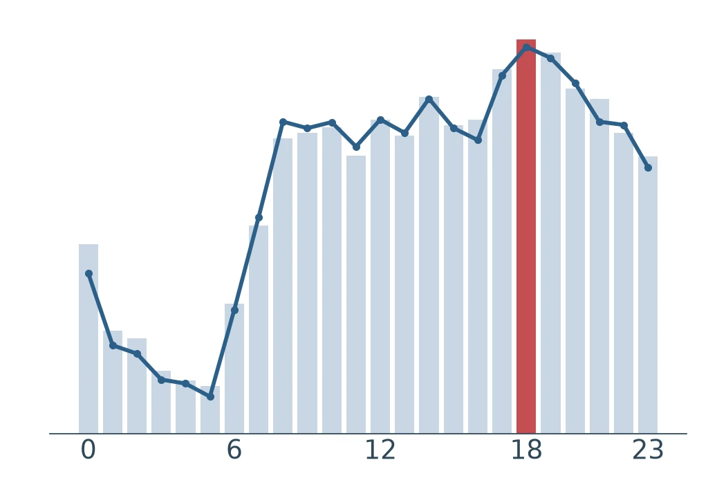
On the projector: set the ranks to the room’s winning entry, usually (3, 3, 1): 60 numbers in place of 480, an 8x saving, at 4.69% error. One hour pattern is left, and it peaks at 18, the hour the notebook printed. The winning entry kept exactly the daily shape the trips are built around. Two tools, one answer. Click a core voxel to show which pickup pattern, dropoff pattern and hour pattern it weights. Switch the view to rebuilt, then to residual, to show what the compression misses.

Kahoot 3 — Convolution & Tensor Decompositions

Active break: Kahoot 3, Convolution & Tensor Decompositions. 6 questions covering convolution, correlation, Tucker and CP. Join at kahoot.it; recognise the structure first, then choose the operator.

Kahoot ↗

Run this right after section 10, while the taxi-tensor rush-hour result is still on screen.

ITS LAST QUESTION NAMES HOUR 18 — it must come AFTER §10’s rank explorer, which prints the busiest hour and the hour Tucker’s first hour pattern peaks at, never before, or it gives the answer away.

NEVER CUT THIS ONE. It checks whether Tucker landed while the taxi result is still on screen. Go straight from the podium into section 11, which takes the same tensor to CP.

11 · Tensor factorizations

IV

15 min

Practise today

Compare CP and Tucker on the same tensor using parameter counts, reconstruction errors, and the budget gap.

Explore later

Study Tensor Train and t-SVD, investigate CP uniqueness, and compress neural-network layers.

Colab ↗

Exercise 1 in pairs (7): CP and Tucker on one budget. Then golf hole 2 (5): the bar drops to 2%, and CP rank 6 wins with 198 numbers against Tucker’s 236. Leaderboard and the budget stage (3), never before the pair exercise, which it would answer.

Explore later

Four decompositions, four bargains. CP stores a sum of rank-1 components, R times I plus J plus K numbers, and is the choice when the components have to be read one by one. Tucker stores one subspace per mode plus a core, and is the choice when each mode needs a rank of its own. Tensor Train stores a chain of small cores, growing only linearly with order, and is the choice when a dense core would explode. And t-SVD takes an FFT along mode 3, matrix SVDs, and an inverse FFT, and is the choice when the third mode carries a meaning of its own.

Colab ↗

📖 CP or Tucker ↗

Optional reference: Tensor Train and t-SVD are outside today’s CP–Tucker comparison. Return to the core activity if teaching live.

Compression golf: hole 2

Any model now. Relative error under 2%; fewest numbers wins.

• golf("cp", 4) or golf("tucker", (4, 4, 3)) prints one scorecard line.
• Hole 1 was won with 60 numbers. This bar costs more.
• Post your best line.

Five minutes to play, then three for the board and the next slide.

Par is CP rank 6: 198 numbers at 1.76%. Tucker’s best is (4, 4, 5), 236 numbers at 1.80%; (4, 4, 4) stores 196 and misses at 2.26%. CP rank 5 misses too, at 2.17%.

Put the two holes side by side on the board. At 7%, Tucker won with 60 numbers against CP’s 66. At 2%, CP wins with 198 against Tucker’s 236. Same tensor, same two models, and the winner flipped. Then open the budget scene.

Predict first: same budget — who wins?

The same parameter budget, spent as CP and spent as Tucker — once the pairs have their own numbers.

Open the budget widget ↗

Hold this for golf’s leaderboard, after the pairs have compared their own CP and Tucker fits: it shows both holes in one picture, and shown earlier it answers the pair exercise for them.

Ask the room to predict before you click: CP rank 3 and Tucker (3, 3, 3) — same cost? They are not: CP rank 3 is 99 numbers, Tucker (3, 3, 3) is 126.

Drag the budget down to 66 parameters: Tucker wins, 4.69% error against CP’s 7.00%. (The notebook’s CP reached 6.73% there; the stage’s fit stops early from one start, as its ALS scene shows.) From 99 numbers on, CP wins instead: hole 1 was won left of that line, hole 2 right of it. The one number to leave the room with: which model wins depends on the budget, not on which one is “better”.

Then put the report’s question to the room: it called CP better at “rank 3”. What did it hold fixed, and what did each model actually store?

Only if a minute is left before the recap: rank has a price outside compression too. Matrix multiplication is a contraction with a fixed tensor of 0s and 1s, and that tensor’s CP rank is the number of multiplications it needs. For 2 × 2 it is 7, Strassen’s, which is why n³ becomes n^2.807. For 3 × 3 it is a 9 × 9 × 9 tensor of 27 ones whose rank nobody knows: somewhere from 19 to 23. Rank 21 would beat Strassen, and DeepMind has pointed AlphaTensor and AlphaEvolve at the problem. The handbook’s Still open note at the end of section 11 has the code and the papers.

One idea connects the workshop

Approximate useful structure when the exact solution is not enough.

Pseudoinverse

Section 07

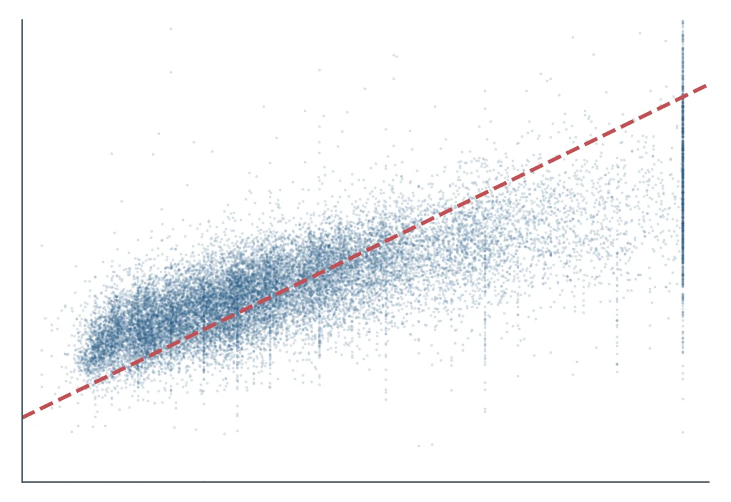
X.shape = (20433, 7): 20,433 equations, 7 unknowns, no exact solution. pinv(X) @ y is the least-squares fit; the dashed line is a perfect prediction.

Tucker

Section 10

480 taxi counts kept as 60 numbers, ranks (3, 3, 1), at 4.69% error. Trips per hour, counted and rebuilt: both peak at 18:00.

Deconvolution

Take-home 13

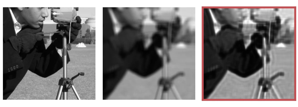
A known 9 × 9 blur, undone approximately: Richardson–Lucy, 20 iterations, 18.9% → 13.1% error. Plausible, not exact.

hard problem → structure → useful approximation

Key idea: we are not always looking for algebraic exactness; we are looking for a representation that preserves what matters.

Colab ↗

Stating this connection explicitly is what makes the second half feel like one lesson rather than four separate blocks. Do not skip it. Section 07’s tensor inverse slide opens it; this is where it closes.

Every number on the slide is one the room printed: X.shape in section 07’s Exercise 2, hole 1’s par in section 10’s golf, and take-home 13’s Exercise 3.

Convolution is the one leg of the three the room no longer runs. Say so, and say that take-home 13 is where it happens to a real photograph.

30-second callback to the cold open, inside this recap: replay the transposed voice from the very first slide. Let the room name the bug — a reshape or transpose done without asking what each axis means. Then switch back to “as the transform built it” and let it play clean. That is the one idea, heard twice.

12 · Wrap-up and take-homes

—

5 min

Practise today

Transfer axis reasoning to new data and explain why Tucker restores shape while losing information.

Explore later

Choose take-home work on PCA, attention, CP, Cholesky, audio, or deep dives 13–16.

Colab ↗

📖 Fourier finally clicked ↗

Collect the five-minute individual exit check before assigning any extensions.