During the live session: follow the notebook’s contiguous core block. The labels below distinguish what you practise today from the reference material you can explore later.
This is the session text: the theory, every exercise, the worked solutions and the take-home appendices. It is what to follow during the workshop and what to keep afterwards. The books and papers behind it are on the references page, which holds them for both languages.
Before you arrive, work through the prerequisites on the workshop homepage: the required reading, the pre-work notebooks, and what to have ready on the day. The homepage also describes every other resource — the slides, the notebooks you type in, the three Kahoot checks and the references.
A note on numbering. This handbook groups the workshop into four Parts and seven exercise Blocks. The notebooks, the slides and the section tables number those same segments 00 to 12, and that number is the canonical one. The schedule below carries both, so any row can be read across to turn one label into the other.
Practise today: Name possible axes and predict a slice in the entry check.
Explore later: After the entry check, revisit data-quality examples. Complete runtime setup before class.
Schedule
| # | Part | Block | Segment | Format | Min | Start |
|---|---|---|---|---|---|---|
| 00 | — | — | Setup and welcome | setup | 5 | 00:00 |
| 01 | I | — | What a tensor is | demo | 20 | 00:05 |
| 02 | II | — | Thinking in N dimensions | demo | 20 | 00:25 |
| 03 | III | 1 | Indexing and broadcasting real data | exercise | 15 | 00:45 |
| 04 | III | 2 | Reshape and transpose real images | exercise | 15 | 01:00 |
| — | 🎯 | — | Kahoot 1 — Tensor Vocabulary & Shapes | quiz | 5 | 01:15 |
| — | — | — | Break | — | 5 | 01:20 |
| 05 | III | — | Video pipeline design | group | 15 | 01:25 |
| 06 | IV | 3 | Contraction with einsum | exercise | 15 | 01:40 |
| — | — | — | Break | — | 5 | 01:55 |
| 07 | IV | 4 | Inverses and the pseudoinverse | exercise | 15 | 02:00 |
| — | 🎯 | — | Kahoot 2 — Einsum, Distance & the Pseudoinverse | quiz | 5 | 02:15 |
| 08 | IV | — | Recursion with matrices and vectors | demo | 10 | 02:20 |
| 09 | IV | 5 | Matrix factorizations | exercise | 15 | 02:30 |
| — | — | — | Break | — | 5 | 02:45 |
| 10 | IV | 6 | Tucker decomposition on real data | exercise | 15 | 02:50 |
| — | 🎯 | — | Kahoot 3 — Convolution & Tensor Decompositions | quiz | 5 | 03:05 |
| 11 | IV | 7 | Tensor factorizations | exercise | 15 | 03:10 |
| 12 | — | — | Wrap-up and take-homes | wrap-up | 5 | 03:25 |
Why the quizzes sit where they do. Each one follows the sections that supply its content, while the material is still fresh. Each also lands before the next context switch — a break, or a new Part. So a quiz reinforces the work rather than interrupting it. Quiz 1 closes out the shape-and-vocabulary work of sections 03 and 04. Quiz 2 closes out the einsum and pseudoinverse stretch, sections 06 and 07. Quiz 3 closes out section 10’s Tucker while the taxi result is still on screen, before section 11 takes the same tensor to CP.
The Data We Use
Included inside the libraries (no download, works offline):
| Dataset | What it is | Shape |
|---|---|---|
load_breast_cancer() |
569 real patients, 30 measurements from tumour cell images | (569, 30) |
load_digits() |
1797 real handwritten digits | (1797, 8, 8) |
data.camera(), data.astronaut() |
Real photographs | (512, 512), (512, 512, 3) |
data.immunohistochemistry(), data.cell() |
Real histology and microscopy images | (512, 512, 3), (660, 550) |
Downloaded once (needs internet, takes a few seconds):
| Dataset | What it is | Used for |
|---|---|---|
| California Housing | 20,640 real housing districts from the 1990 US census | Pseudoinverse, least squares |
| NYC Taxi Trips | 6,433 real taxi journeys in New York | Tensor factorization |
| Airline Passengers | 144 months of real airline traffic, 1949–1960 | Recursion, forecasting |
Every code snippet in this handbook assumes the names notebook 00’s setup cell binds, so if you are reading along outside a notebook, start here:
import numpy as np
import pandas as pd
from sklearn.datasets import load_digits, load_breast_cancer
from skimage import data
from scipy import signal
from scipy.linalg import lu, toeplitz

HOUSING = "https://raw.githubusercontent.com/ageron/handson-ml2/master/datasets/housing/housing.csv"
TAXIS   = "https://raw.githubusercontent.com/mwaskom/seaborn-data/master/taxis.csv"
FLIGHTS = "https://raw.githubusercontent.com/mwaskom/seaborn-data/master/flights.csv"
Notebook 00 downloads all three and prints their shapes — (20640, 10) (6433, 14) (144, 3). Run it in Colab before the session. If it fails, say so in Discord at once: a download that fails quietly leaves you stuck at sections 07 and 10, an hour in. Every other notebook loads only the data its own section needs, so you can open any one of them cold.
PART I — What a Tensor Is (section 01, 20 min)
Practise today: Name image axes and distinguish shape, order, and element count.
Explore later: Extract slices and fibers, and unfold images into matrices.
1.1 Vocabulary
Keep this table open from section 00 to section 12.
| Term | Plain meaning | Spanish | Example |
|---|---|---|---|
| Tensor | An array of numbers with any number of axes | tensor | A colour image |
| Axis (pl. axes) | One direction along which data is arranged | eje | Height; width; colour |
| Mode | Another word for axis, used in tensor theory | modo | “mode-0 unfolding” |
| Order | How many axes a tensor has | orden | A matrix has order 2 |
| Shape | The size along each axis, as a tuple | forma | (512, 512, 3) |
| Slice | Fix one index, keep the rest | corte | One colour channel |
| Fiber | Fix every index except one | fibra | The 3 colour values of one pixel |
| Unfolding | Rearranging a tensor into a matrix | desplegado | Needed for decompositions |
| Contraction | Multiply and sum over a shared axis | contracción | The dot product |
| Decomposition | Writing one tensor as a product of simpler ones | descomposición | SVD, PCA, Tucker |
⚠️ Warning about the word “rank”. In Chapter 2, rank means the number of independent columns of a matrix. In tensor theory, rank often means the number of axes. To avoid confusion, this workshop says order for the number of axes, and rank only in Chapter 2’s sense.
1.2 Shape in NumPy
Every NumPy array has .shape, a tuple giving the size along each axis. The length of that tuple is .ndim, the number of axes.
scalar = np.array(3.0)                     # book: a           — order 0
vector = np.array([1., 2., 3.])            # book: x, x_i      — order 1
matrix = np.array([[1., 2.], [3., 4.]])    # book: A, A_{i,j}  — order 2
tensor = np.random.randn(2, 3, 4)          # book: A_{i,j,k}   — order 3

for name, arr in [("scalar", scalar), ("vector", vector),
                  ("matrix", matrix), ("tensor", tensor)]:
    print(f"{name:8s} shape={str(arr.shape):12s} ndim={arr.ndim}  size={arr.size}")

# scalar   shape=()          ndim=0  size=1
# vector   shape=(3,)        ndim=1  size=3
# matrix   shape=(2, 2)      ndim=2  size=4
# tensor   shape=(2, 3, 4)   ndim=3  size=24
A scalar has shape=(), an empty tuple — there are no axes to measure. And size is always the product of the numbers in shape: 2 × 3 × 4 = 24.
Now with real data:
digits = load_digits()
print(digits.images.shape)      # (1797, 8, 8)  — 1797 handwritten digits, 8x8 pixels

photo = data.immunohistochemistry()
print(photo.shape)               # (512, 512, 3) — height, width, colour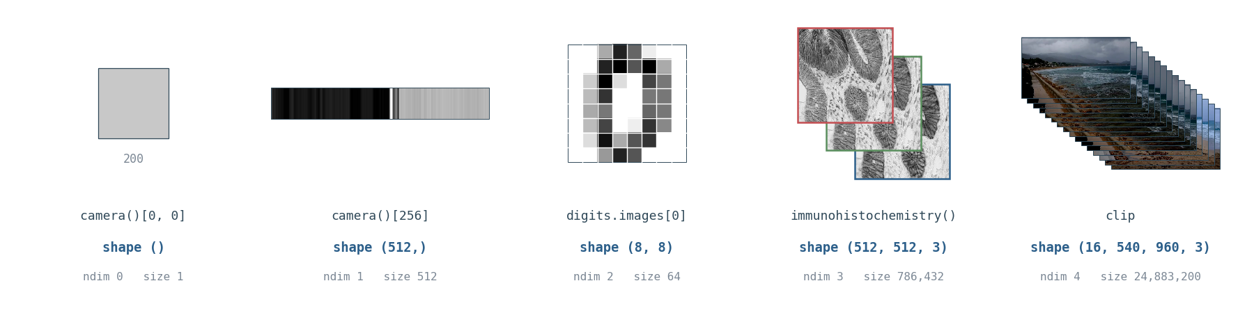
The same climb, in arrays you will meet today. shape grows by one number at each rung; the last two rungs both have a 3 in them, and the two threes mean nothing like each other.
Both are order 3, but their axes mean completely different things. digits.images counts images along axis 0; photo counts colours along axis 2. The shape alone never tells you what the axes mean. You must know, and you must keep track.
1.3 The Three Operations That Matter
Slices and fibers — fixing indices takes a tensor apart.
photo[:, :, 0].shape       # (512, 512) — a slice: one colour channel, still an image
photo[100, 200, :].shape   # (3,)       — a fiber: the 3 colour values of one pixel
Unfolding — every tensor decomposition begins by turning the tensor into a matrix, one axis at a time. Move axis k to the front, then flatten the remaining axes into one long axis.
def unfold(T, axis):
    return np.moveaxis(T, axis, 0).reshape(T.shape[axis], -1)

print(unfold(photo, 0).shape)   # (512, 1536) — rows are the height axis
print(unfold(photo, 2).shape)   # (3, 262144) — rows are the 3 colour channels
Unfolding loses nothing. It only rearranges. The mode-2 unfolding says “each colour channel is one row of 262,144 numbers”. Every matrix tool you know, SVD included, now applies to it.
Contraction — multiply along a shared axis and sum over it. The dot product (eq. 2.8) and the matrix product (eq. 2.5) are both contractions. np.einsum writes them directly:
a = np.array([1., 2., 3.]); b = np.array([4., 5., 6.])
np.einsum('i,i->', a, b)          # dot product, sum over i          (eq 2.8)

A = np.array([[1., 2.], [3., 4.]]); B = np.array([[5., 6.], [7., 8.]])
np.einsum('ik,kj->ij', A, B)      # matrix product, sum over k       (eq 2.5)
The rule, in one sentence: an index that appears in the inputs but not after the arrow is summed over. An index that appears after the arrow is kept.
1.4 The Map of Factorizations
A factorization writes one object as a product of simpler objects. You met two in Chapter 2. Here are the eight we will use today:
| Method | Works on | What it gives you | Where today |
|---|---|---|---|
| LU | Square matrix | Gaussian elimination, saved for reuse | Below |
| QR / Gram-Schmidt | Any matrix | Perpendicular, unit-length directions | Below |
| Eigendecomposition | Square matrix | Directions that only get scaled (§2.7) | Recursion demo |
| SVD | Any matrix | The most general matrix factorization (§2.8) | sections 07 and 10 |
| PCA | Data matrix | Compression to fewer features (§2.12) | Take-home A |
| Pseudoinverse | Any matrix | “Inverse” when no true inverse exists (§2.9) | section 07 |
| Cholesky | Symmetric positive-definite matrix | A “square root” of a covariance matrix, for building correlated data | Appendix D |
| Tucker / CP | Tensor, any order | PCA generalized to every axis | section 10 |
Today uses each of these where it happens to be needed. Section 09 puts six factorizations side by side — five from this table, plus NMF — and asks what each one costs. This table does not answer that question.
A = np.array([[4., 3., 2.], [2., 1., 1.], [6., 3., 5.]])

P, L, U = lu(A)                            # LU: A = P L U
print(np.allclose(P @ L @ U, A))            # True

Q, R = np.linalg.qr(A)                      # QR: orthonormal directions
print(np.allclose(Q.T @ Q, np.eye(3)))      # True — book eq 2.37
LU is Gaussian elimination stored as two triangular matrices, so Ax = b can be solved cheaply many times for different b. QR (computed by Gram-Schmidt, or more stably by other methods) produces orthonormal directions — mutually perpendicular, each of length 1. It is used for orthogonal weight initialization in neural networks and for stable least-squares.
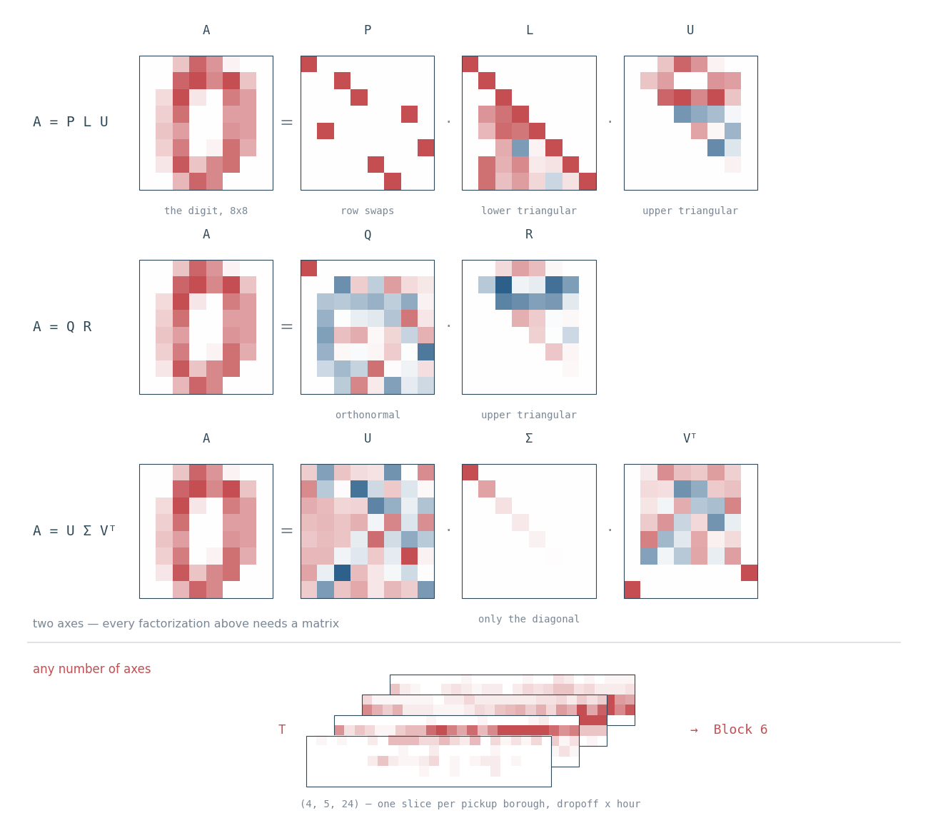
The same 8×8 digit, factorized three ways. The shapes are the point: L really is lower triangular, U upper, and Σ is empty apart from its diagonal. Below the line is an object none of them can touch.
Every method in that table above the double line works on matrices — two axes. Real data often has more. That is what section 10 addresses.
PART II — Thinking in N Dimensions (section 02, 20 min)
Practise today: Keep images and labels paired when shuffling; explain why shuffling time changes a sequence.
Explore later: Build padded video batches and interpret additional experimental axes.
A live coding demo in the notebook, on real image and video tensors. Open it in Colab and run the Setup cell first — it downloads and checksums the real video clip used by the exercises. Three exercises:
- Read the axes on real tensors.
digits.imagesis(1797, 8, 8)and a photo is(512, 512, 3). Both are order 3. But axis 0 counts whole images in one, and rows of pixels in the other.digit_batchandvideo_patchare both(8, 8, 8). Before you run a line of code, say what every axis counts. - Shuffle a batch vs shuffle time. Shuffling axis 0 is harmless for a batch: examples are independent, and order carries no information. It destroys a video, where order is the information. The same operation, a completely different meaning. Chapter 2’s notation has no concept of “order matters between elements.” That is genuinely new today.
- Batch clips of different lengths. Real videos have different frame counts, but a batch tensor is rectangular. Take three real clips of length 4, 7 and 5 and pad them into one
(3, 7, 135, 240, 3)order-5 batch. Carry a Boolean(3, 7)validity mask alongside it, sovalid.sum() == 16. The padding then stays visible instead of being averaged into the data.
PART III — Working With Tensor Axes (sections 03–05)
03 · Indexing and Broadcasting Real Data (Block 1, 15 min)
Practise today: Predict broadcasting shapes and standardize pixel columns safely when variance is zero.
Explore later: Select observations with named features, fancy indexing, and Boolean masks.
Why this matters. The breast_cancer data holds 30 real measurements of tumour cell nuclei for 569 real patients. Selecting the wrong column produces no error. It returns a different real measurement, your analysis continues, and it gives a confident, wrong answer. In research this produces results nobody can reproduce. In a clinical tool it produces a wrong recommendation about a real person.
In tech, the identical operation runs on a (users, items) matrix to pull one user’s history before making a recommendation.
Exercise (10 min)
bc = load_breast_cancer()
X, y = bc.data, bc.target          # (569, 30); y: 0 = malignant, 1 = benign
names = list(bc.feature_names)

# TODO 1: Print X.shape. Say out loud what each axis means.
# TODO 2: Extract the column "mean radius" for all patients -> shape (569,).
#         Find its position with names.index(...). Do not hard-code a number.
# TODO 3: Find the 5 patients with the LARGEST mean radius, then extract their
#         full 30-measurement profiles as one (5, 30) array, in ONE operation.
# TODO 4: Using boolean indexing, compare mean radius for malignant (y == 0)
#         against benign (y == 1) patients. Is there a real difference?

# --- broadcasting, on real images ---
images = load_digits().images          # (1797, 8, 8)
D = images.reshape(len(images), -1)    # (1797, 64)

# TODO 5: Compute the mean and std of each of the 64 pixels across all images.
# TODO 6: Standardize with broadcasting: (D - mean) / std.
#         RUN IT AND LOOK AT THE RESULT before continuing.
# TODO 7: You will find NaN. How many pixels have std == 0, and why would a real
#         handwritten digit image contain such pixels? Fix it, then verify no NaN.
Explanation (5 min)
i = names.index("mean radius")
radius = X[:, i]                                   # book notation A_{:,j}
top5 = np.argsort(radius)[-5:]
profiles = X[top5, :]                               # (5, 30)
print(radius[y == 0].mean(), radius[y == 1].mean()) # 17.5 vs 12.1

mean, std = D.mean(axis=0), D.std(axis=0)
print((std == 0).sum())                             # 3
Z = (D - mean) / np.where(std == 0, 1.0, std)
Two real results. Malignant tumours really do have a larger mean radius — 17.5 against 12.1. And three pixels are always dark in all 1797 digit images: they sit in corners where nobody writes. Their standard deviation is exactly zero, so dividing produces NaN. Random data would never have shown you this.
The shape rule has its own page: the broadcasting simulator lines two shapes up from the right and steps through the stretch. Try (4, 5) against (4,), then against (4, 1).
04 · Reshape and Transpose Real Images (Block 2, 15 min)
Practise today: Convert HWC to CHW and test that pixel values keep their meaning.
Explore later: Build image batches, compare NHWC with NCHW, and inspect memory layout.
Why this matters. Microscopes and cameras order their axes according to the hardware, not according to what a model expects. Getting this wrong does not crash — the model runs on scrambled data and returns confident, meaningless output. In a drug screen, that is a wrong decision about whether a compound works. The famous version in tech: a model trained in TensorFlow (NHWC) deployed into PyTorch (NCHW) with no transpose.
Exercise (10 min)
photo = data.immunohistochemistry()   # (512, 512, 3) real histology
cells = data.cell()                    # (660, 550)    real microscopy, grayscale

# TODO 1: Print both shapes. Which one has no colour axis?
# TODO 2: Convert `photo` from (H, W, C) to (C, H, W) with np.transpose.
# TODO 3: Stack `photo` three times into a batch of shape (3, 512, 512, 3).
#         Which axis is the batch axis?
# TODO 4: Convert that batch from NHWC to NCHW -> (3, 3, 512, 512).
#         Two axes now both have size 3. How do you know which is which?
# TODO 5: photo.reshape(3, 512, 512) runs WITHOUT error but is wrong.
#         Run it, compare against TODO 2, and explain the difference.
Explanation (5 min)
chw   = np.transpose(photo, (2, 0, 1))      # (3, 512, 512) — correct
batch = np.stack([photo, photo, photo])      # (3, 512, 512, 3)
nchw  = np.transpose(batch, (0, 3, 1, 2))    # (3, 3, 512, 512)
wrong = photo.reshape(3, 512, 512)           # runs, but scrambles the image
Reshape only reinterprets numbers in memory order. Transpose moves them according to axis meaning. Both give shape (3, 512, 512); only one is the image. And TODO 4 makes the deeper point: once two axes share a size, the shape cannot tell you which is which. Only your own tracking can.
The three photographs above are cubes, one per byte, on the image tensor visualizer. Transpose NHWC to NCHW and watch the cubes follow the new shape while the buffer strip under them does not move a byte; then compare with reshape and watch the picture break.
Kahoot Quiz 1 — Tensor Vocabulary & Shapes (5 min)
Run this before the break, right after section 04. The room has just used order, axis, shape, variance, reshape and transpose. This is the moment those words are freshest. One question asks what fixing every index but one gives you, a fiber, which only section 01’s Explore later covers. Give the one-line definition as its answer is revealed. Launch kahoot_quiz_1_vocabulary_shapes.xlsx (6 questions, ~5 min including the podium). No prep needed beyond having it imported into a kahoot ahead of time.
Break (5 min)
05 · Group Exercise — Video Pipeline Design (15 min)
Practise today: Trace sampled frames to source indices and defend a sampling strategy for a brief event.
Explore later: Compare complete pipelines, padding costs, and synchronized-camera layouts.
The live slot is notebook 05’s core, not this design exercise: a one-minute Myth or fact round, the opening prediction and Exercise 1 (6 minutes together), then group task 05, keep the event, fit the budget, for 8 minutes, with its three-line share-back posted in Discord. The five questions below are the take-home version of the same problem. There is no single correct answer.
Design the tensor shape at each stage — raw file → decoded frames → preprocessed batch → model input → model output — for both systems: - Tech: a short-video app computing one embedding per video from sampled frames, to choose what to play next. - Biotech: a surgical-video model that labels the current phase of an operation from an operating-room camera.

Both panes hold the same eight frames, the same shape and the same sum. Only the order of axis 0 differs, and no arithmetic in this workshop can tell you which one is the video.
- Sketch the shape at each of the five stages, for both. Where are they the same, and where must they differ?
- Clips have different lengths — 30 seconds against 4 hours. Take the padding-and-mask strategy from Part II and give the exact shape of the preprocessed batch. What does an invented or wasted value in that tensor represent?
- The surgical system adds three camera angles recording at once. Where does that axis go, and why does its position change how easy the rest of the pipeline is to write?
- The recommender samples 8 frames out of 900. Which operation from section 03 does that, and what is lost?
- Both systems must decide which frames matter most. What kind of mechanism could learn that weighting?
PART IV — Computing With Tensors (sections 06–11)
06 · Contraction With einsum (Block 3, 15 min)
Practise today: Contract colour with einsum, name surviving axes, and verify a weighted pixel sum.
Explore later: Express matrix operations with einsum and compare digit similarity measures.
Why this matters. Recommendation and search systems rank items by the dot product between a user vector and every item vector. That is one user against millions of items, many times per second. That contraction is the ranking signal. Sum over the wrong axis and every user gets wrong results.
Exercise (10 min)
photo = data.immunohistochemistry().astype(float)        # (512, 512, 3)
batch = np.stack([photo, data.astronaut().astype(float)]) # (2, 512, 512, 3)
w = np.array([0.2125, 0.7154, 0.0721])                    # RGB -> grayscale weights

# TODO 1: With einsum, convert `photo` to grayscale by contracting the colour
#         axis against w. Result shape (512, 512).
# TODO 2: Do the same for the whole batch in ONE einsum call -> (2, 512, 512).
# TODO 3: Write these Chapter 2 operations as einsum and check each against NumPy:
#           (a) trace          (eq 2.48)
#           (b) transpose      (eq 2.3)
#           (c) matrix product (eq 2.5)
# TODO 4: Flatten the digits to (1797, 64) and compute the (1797, 1797) similarity
#         matrix between every pair of digit images with one einsum.
Explanation (5 min)
gray       = np.einsum('hwc,c->hw',   photo, w)     # (512, 512)
gray_batch = np.einsum('nhwc,c->nhw', batch, w)      # (2, 512, 512)

np.einsum('ii->', A)           # trace          == np.trace(A)
np.einsum('ij->ji', A)         # transpose      == A.T
np.einsum('ik,kj->ij', A, B)   # matrix product == A @ B
c appears in the inputs but not after the arrow, so it is summed over — that is the contraction. n, h, w appear after the arrow, so they are kept. Adding a batch axis costs exactly one letter. This is why einsum is worth learning. The same expression works for one image or for a million, and it reads like the mathematics in Chapter 2. Attention is two more contractions of exactly this shape — L = Q Kᵀ sums over the feature axis, O = A V sums over the key axis — on the attention stage’s scores and output pictures.
07 · Inverses and the Pseudoinverse (Block 4, 15 min)
Practise today: Show how duplicate columns give identical predictions from different coefficients; explain the minimum-norm choice of pinv.
Explore later: Verify the four Moore–Penrose identities, fit housing data, and apply pinv to unfolded images.
Live core: what can the coefficients tell us?
Use three deliberately synthetic observations: x = [1, 2, 3], duplicate the feature to make A = [x, x], and set y = 2*x. Coefficients [2, 0] and [0, 2] both reproduce y. Every row depends only on the sum of the coefficients, so these observations cannot identify the separate effects.
Compute pinv(A) @ y: it selects [1, 1]. All exact solutions have the form [1+t, 1-t], with squared norm 2 + 2*t**2, minimized at t=0. Minimum norm is a mathematical selection rule; it does not establish equal real effects. With noisy observations, pinv selects the minimum-norm solution among the least-squares minimizers.
Attempt: construct a different coefficient vector with the same predictions, compare norms, and explain what remains unknown. Follow the contiguous notebook core for feedback and its checkpoint.
Explore later: the theory and housing exercises below, including the four Moore–Penrose identities, extend the live activity.
The theory, in three steps
Step 1 — square matrices. Chapter 2 §2.3 defines A⁻¹ for a square matrix, with A⁻¹A = I. But this only exists when the columns are linearly independent. A matrix with dependent columns is singular and has no inverse:
S = np.array([[2., 1.], [1., 3.]])
np.linalg.inv(S) @ S                       # ≈ identity, fine

Singular = np.array([[1., 2.], [2., 4.]])  # column 2 = 2 × column 1
np.linalg.inv(Singular)                     # raises LinAlgError
Step 2 — non-square matrices. A⁻¹ is not even defined. But we still need to solve Ax = b. In machine learning A is almost never square: it has one row per example and one column per feature, and there are always far more examples than features.
The Moore-Penrose pseudoinverse A⁺ (Chapter 2 §2.9) is the answer. It is defined for every matrix — square or not, singular or not — and it is computed from the SVD (eq. 2.47):
A = np.random.randn(5, 3)
A_plus = np.linalg.pinv(A)
print(A.shape, A_plus.shape)               # (5, 3) (3, 5) — note the shape flips

U, S_, Vt = np.linalg.svd(A, full_matrices=False)
print(np.allclose(A_plus, Vt.T @ np.diag(1/S_) @ U.T))   # True — this is eq 2.47
It satisfies four conditions that define it uniquely — all verified to be True:
np.allclose(A @ A_plus @ A, A)            # 1
np.allclose(A_plus @ A @ A_plus, A_plus)  # 2
np.allclose((A @ A_plus).T, A @ A_plus)   # 3
np.allclose((A_plus @ A).T, A_plus @ A)   # 4
What A⁺ gives you depends on the shape, exactly as Chapter 2 §2.9 says: - More rows than columns (too many equations, usually no exact solution) → x = A⁺b gives the x that makes Ax as close as possible to b. This is least squares. - More columns than rows (too few equations, infinitely many solutions) → x = A⁺b gives the valid solution with the smallest norm.
Step 3 — what about tensors? This is a fair question with an honest answer. No single tensor inverse is in common use. Several definitions exist — built on the Einstein product, or on the t-product for order-3 tensors — and they are active research. In practice, in machine learning, you unfold the tensor into a matrix, use the matrix pseudoinverse, and fold the result back. That works because unfolding loses nothing:
T = np.random.randn(4, 3, 5)
M = unfold(T, 0)                       # (4, 15)
M_plus = np.linalg.pinv(M)             # (15, 4)
np.allclose(M @ M_plus @ M, M)          # True
This is a general lesson worth remembering: when a tensor problem is hard, unfold it to a matrix, solve it there, and fold back.
Exercise (10 min) — real California housing data.
# Predict house value from district features. 20,640 real districts.
print(housing.shape)                                   # (20640, 10)
print(housing['total_bedrooms'].isnull().sum())         # 207 missing values!

# TODO 1: Drop rows with missing values. How many rows remain?
# TODO 2: Build X from these columns, and add a column of ones for the bias:
#         ['housing_median_age','total_rooms','total_bedrooms',
#          'population','households','median_income']
#         Target y = 'median_house_value'. Print X.shape. Is X square?
# TODO 3: Try np.linalg.inv(X). What happens, and why?
# TODO 4: Solve for the weights with the pseudoinverse: w = pinv(X) @ y.
# TODO 5: Check your answer against np.linalg.lstsq. Do they agree?
# TODO 6: Compute the RMSE of the predictions. Which feature has the largest
#         coefficient, and does that make sense for house prices?
Explanation (5 min)
d = housing.dropna()                                     # 20433 rows remain
feats = ['housing_median_age','total_rooms','total_bedrooms',
         'population','households','median_income']
X = np.column_stack([np.ones(len(d)), d[feats].to_numpy(float)])   # (20433, 7)
y = d['median_house_value'].to_numpy(float)

w = np.linalg.pinv(X) @ y
w_lstsq, *_ = np.linalg.lstsq(X, y, rcond=None)
np.allclose(w, w_lstsq)                                   # True

rmse = np.sqrt(((X @ w - y) ** 2).mean())                 # ≈ 75,980
X is 20433 × 7 — very tall, so np.linalg.inv cannot even be called. There is no exact solution: no straight line passes through 20,433 points. The pseudoinverse gives the best possible answer instead. lstsq agrees with it exactly, because it solves the same problem. The largest coefficient belongs to median_income (about 47,700 per unit), which is the sensible result — income predicts house prices.
That geometry has its own page: the projection and SVD stage takes three of these districts and two predictors, so the column space is a plane you can see, and draws ŷ as the closest point on it with the residual meeting it at a right angle. Slide y off the plane and watch β refuse to move — least squares cannot see the direction it is throwing away.
Kahoot Quiz 2 — Einsum, Distance & the Pseudoinverse (5 min)
Run this right after section 07, before the recursion demo. It covers contraction (section 06’s einsum), the pseudoinverse and singular matrices (section 07), and distance and similarity. The digit-similarity matrix from section 06 TODO 4 is the natural bridge between the two. Launch kahoot_quiz_2_distance_pseudoinverse.xlsx (6 questions, ~5 min).
08 · Recursion With Matrices and Vectors (10 min — demo)
Practise today: Explain a matrix state update and connect repeated updates with a matrix power.
Explore later: Use power iteration and evaluate recursive forecasts on airline traffic.
Recursion means defining something in terms of itself. With matrices this becomes: apply the same matrix again and again. Three examples, increasing in usefulness.
1. Fibonacci as repeated matrix multiplication. The rule f(n) = f(n-1) + f(n-2) is one matrix applied repeatedly:
F = np.array([[1, 1], [1, 0]])
v = np.array([1, 0])
for _ in range(10):
    v = F @ v
print(v[1])                                  # 55
print(np.linalg.matrix_power(F, 10)[0, 1])   # 55 — same answer, one step
2. Power iteration — recursion that finds an eigenvector. Multiply any starting vector by A repeatedly, rescaling each time. It converges to the eigenvector with the largest eigenvalue (Chapter 2 §2.7):
A = np.array([[4., 1.], [2., 3.]])
x = np.random.randn(2); x /= np.linalg.norm(x)
for _ in range(50):
    x = A @ x
    x /= np.linalg.norm(x)

print(x @ A @ x)                    # 5.000000
print(np.linalg.eig(A)[0].max())    # 5.000000 — identical
This is how PageRank ranks web pages. It is also why eigenvectors matter far beyond Chapter 2: repeated application of a matrix converges to its dominant eigenvector. The eigenvector step of the projection and SVD stage draws the test itself: a field of arrows under A, with the ones that kept their direction lit.
3. Recursion on real data — forecasting airline traffic. This combines recursion with the pseudoinverse from section 07. We fit a model that predicts each month from the previous 12, then apply it to its own output to forecast forward:
y = flights['passengers'].to_numpy(float)     # 144 real months, 1949–1960
p = 12
rows = np.array([y[i:i+p] for i in range(len(y) - p)])
X = np.column_stack([np.ones(len(rows)), rows])
w = np.linalg.pinv(X) @ y[p:]                  # least squares, exactly as in section 07

history = list(y[-p:])
for _ in range(12):                             # recursion: feed predictions back in
    nxt = w[0] + np.dot(w[1:], history[-p:])
    history.append(nxt)

print(np.round(history[-12:], 1))
# [465.2 429.1 455.1 491.0 527.8 589.4 679.7 661.3 575.3 509.5 438.6 470.7]
The forecast reproduces the seasonal shape of real air travel, low in winter and peaking in summer. It learned that shape from 132 real training windows. This is exactly the structure of a recurrent neural network: a hidden state, updated by the same weights at every step.
W, U = np.random.randn(4, 4) * 0.5, np.random.randn(4, 3) * 0.5
h = np.zeros(4)
for t in range(6):
    h = np.tanh(W @ h + U @ xs[t])    # same W and U every step — that is the recursion
09 · Matrix Factorizations: Which One, and What It Costs (Block 5, 15 min)
Practise today: Compare solver residuals and coefficient sensitivity; trace reduced coordinates through reconstruction.
Explore later: Benchmark other factorizations, compress images with SVD, and inspect NMF factors.
Part I §1.4 drew the map. Sections 03 to 08 used three of the factorizations on it in passing: LU and QR in §1.4 itself, and the pseudoinverse in section 07. None of them answered the two questions a practitioner actually has: which one do I reach for on this data, and what does it cost me? This section answers both. It is also where eigendecomposition finally gets named, an hour before section 10 leans on the same machinery. The notebook is 09 · Matrix factorizations.
The organizing idea is that all six are constrained optimizations, and the constraint is what gives each factorization its shape. QR minimizes ‖y − Xβ‖ subject to an orthonormal Q. The truncated SVD minimizes ‖A − B‖_F subject to rank(B) ≤ k, and Eckart–Young–Mirsky proves nothing else does better. NMF minimizes the same quantity subject to W, H ≥ 0. That extra constraint must be worse on error, and it is chosen anyway, because the components come out as parts you can name. Cholesky and LU optimize nothing at all. They are exact rewrites, and their value is all downstream, where a solve costs O(n²) instead of O(n³).
The cost table. Leading-term flop counts for a dense m × n factorization with m ≥ n, from Trefethen & Bau, Numerical Linear Algebra:
| Method | Flops | The question it answers |
|---|---|---|
Cholesky (n × n SPD) |
n³/3 |
Solve Ax = b many times, A symmetric positive definite |
LU (n × n) |
2n³/3 |
The same, A merely square |
QR (m × n) |
2mn² − 2n³/3 |
Least squares, without forming XᵀX |
Eigendecomposition (n × n sym.) |
≈ 9n³ |
What does repeated application converge to? |
Thin SVD (m × n) |
2mn² + 11n³ |
The best rank-k approximation of anything |
Randomized SVD (rank k) |
≈ 4mnk |
The same, when k ≪ n and A is dense |
Lanczos (rank k, sparse) |
O(k · nnz(A)) |
The same, when A is sparse |
Three consequences are worth stating outright, because each one is a mistake that costs a single line of code:
- Factor once, solve many. Cholesky costs
n³/3once; each later solve is two triangular substitutions atO(n²). Somright-hand sides costO(n³ + mn²), notO(mn³).np.linalg.inv(A) @ Bis both slower and less accurate than factoring, and is never the right call. - The normal equations square the condition number, because
κ(XᵀX) = κ(X)². QR’s error scales withκ(X)·ε; the normal equations’ withκ(X)²·ε. Same data, same objective, error squared. - Do not compute what you will throw away. A full SVD is
O(mn·min(m,n)). If you want 20 components out of 1682, randomized SVD isO(mnk)and Lanczos isO(k·nnz(A)). That gap is why large-scale recommenders are feasible at all.
The same page carries the other half of this: its SVD portal puts the unit circle and its image side by side, so A vᵢ = σᵢ uᵢ is something you scrub to rather than something you are told, and σ₁/σ₂ is a shape on the screen rather than a ratio. The ellipsoid after it is the same picture one dimension up, and the two steps after that, collinear and float32, are the two consequences above drawn: β swinging out and back as two columns close on each other, and the normal equations dividing by exactly zero once a number format can no longer tell them apart.
The audio tensor stage carries the other two factorizations in this table, both measured rather than quoted. Low rank factors Appendix E’s own (513, 465) matrix in your browser and rebuilds the SNR curve rung by rung as it goes, so the wait is the cost this section keeps asking about. Parts you can name fits NMF to the same kind of matrix and prints its error beside the truncated SVD’s at the same rank — worse, as Eckart–Young says it must be — then lets you solo one component and hear what that fraction of a percentage point bought.
# TODO 1: Fit a degree-10 polynomial to the real airline series two ways.
#         X = np.vander(month_scaled, 11, increasing=True); y = passengers
#         a) normal equations: np.linalg.solve(X.T @ X, X.T @ y)
#         b) QR: Q, R = np.linalg.qr(X); np.linalg.solve(R, Q.T @ y)
#         Use np.linalg.lstsq as the reference. Compare the RESIDUALS, then
#         compare the COEFFICIENTS. Only one of those two comparisons sees
#         the problem.
# TODO 2: Build the 1797x1797 RBF kernel matrix of the digits plus a ridge
#         term, and 200 right-hand sides. Time three strategies: factor once
#         with cho_factor/cho_solve, np.linalg.inv(G) @ B, and one
#         np.linalg.solve per column. Print the ratios, and the relative
#         residual of the first two. Which is both faster AND more accurate?
# TODO 3: Time Cholesky, LU, QR, eigh and SVD across n = 128 ... 768. Fit
#         log t against log n; the slope is the measured exponent. Compare
#         it against the predicted 3, and compare the measured SVD/Cholesky
#         ratio against the 39x the table above predicts. Which of the two
#         predictions survives contact with a real machine?
# TODO 4: Write needed_rank(A, target_db) returning the smallest k whose
#         rank-k truncation reaches a target PSNR — WITHOUT rebuilding the
#         truncation for each k. Eckart-Young gives the squared error as
#         sum(S[k:] ** 2) directly. Run it on the 512x512 astronaut image
#         for 20, 25, 30 and 35 dB and report what each rank costs to store.
Solution
X = np.vander(month_scaled, 11, increasing=True)                   # TODO 1
beta_normal = np.linalg.solve(X.T @ X, X.T @ passengers)
Q, R = np.linalg.qr(X); beta_qr = np.linalg.solve(R, Q.T @ passengers)
beta_ref = np.linalg.lstsq(X, passengers, rcond=None)[0]
# cond(X) = 2.2e+07, cond(X.T @ X) = 4.6e+14 — the square, to one digit
# residuals agree to six decimals; coefficient errors are 2.0e-03 vs 2.0e-14

X_fast = cho_solve(cho_factor(G), B)                               # TODO 2
# factor once = 1x; explicit inverse ~5x slower; one solve per column ~340x
# and the explicit inverse is also ~7x less accurate on the residual

slope, _ = np.polyfit(np.log(sizes), np.log(times), 1)             # TODO 3
# fitted slopes land near 2.2-2.9, not 3.0; and the measured SVD/Cholesky ratio lands well under the predicted 39x

S = np.linalg.svd(A, compute_uv=False)                             # TODO 4
tail = np.concatenate([np.cumsum(S[::-1] ** 2)[::-1], [0.0]])
with np.errstate(divide="ignore"):        # the last entry is exactly 0
    db = 10 * np.log10(1.0 / (tail / A.size))
k = int(np.argmax(db >= target_db))
TODO 1 is the expensive one. The residuals of the two fits agree to six decimal places, so the check most people run reports no problem. Meanwhile the coefficients differ by eleven orders of magnitude. That gap is exactly κ(X)² against κ(X), and it came from writing X.T @ X.
TODO 3 does not give you 3.0, and that is not a failure of the theory. Fitted exponents come in low because parallelism and cache reuse both improve as n grows. The machine gets faster at the same work, and that flattens the curve. The effect shrinks with larger n, so the slope creeps upward. What does survive is the ratio between methods at fixed n. It cancels the machine out, because both methods gain from the same hardware. Predict with ratios, not exponents.
uint8 image: 6.3% of the pixel count, but 12.5% of the bytes at int16 and 25% at float32. Truncated SVD is a superb analysis tool and a mediocre image codec.
Break (5 min)
10 · Tucker Decomposition on Real Data (Block 6, 15 min)
Practise today: Explain core and factor shapes, measure storage and error, and choose Tucker ranks against an error limit.
Explore later: Implement HOSVD and inspect unfoldings, core interactions, and rank sweeps.
The theory
PCA compresses a matrix — two axes. Real data often has more. Tucker decomposition generalizes PCA to a tensor of any order: one factor matrix per axis, plus a small core tensor describing how the factors combine.
The way to compute it, called HOSVD, uses only tools you already have: 1. Unfold the tensor along each axis (Part I). 2. Run SVD on each unfolding; keep the top components. These are the factor matrices. 3. Contract the original tensor against all factor matrices to get the core (section 06).
The related CP decomposition instead writes the tensor as a sum of simple rank-1 pieces. Tucker is usually more accurate at the same size; CP is often easier to interpret.
Our real tensor. From 6,433 real New York taxi trips we build a genuine order-3 tensor: pickup borough × dropoff borough × hour of day.
Exercise (10 min)
taxis['hour'] = pd.to_datetime(taxis['pickup']).dt.hour
sub = taxis.dropna(subset=['pickup_borough', 'dropoff_borough'])
pb = sorted(sub['pickup_borough'].unique())
db = sorted(sub['dropoff_borough'].unique())

T = np.zeros((len(pb), len(db), 24))
for (p, d, h), v in sub.groupby(['pickup_borough','dropoff_borough','hour']).size().items():
    T[pb.index(p), db.index(d), h] = v

# TODO 1: Print T.shape and T.sum(). What does the entry T[i, j, k] mean?
# TODO 2: Which hour has the most trips overall? (Sum over the first two axes.)
# TODO 3: Unfold T along each axis and print the three shapes. Confirm the total
#         number of entries is the same each time — unfolding loses nothing.
# TODO 4: Run SVD on each unfolding, keep the top (2, 2, 3) components, and build
#         the core tensor with ONE einsum call.
# TODO 5: Reconstruct T from the core and factors, again with one einsum.
#         Compute the relative error and the compression ratio.
# TODO 6: Look at the first column of the hour factor matrix. At which hour is it
#         largest? Does that match what you found in TODO 2?
Explanation (5 min)
Us = [np.linalg.svd(unfold(T, ax), full_matrices=False)[0] for ax in range(3)]
r = (2, 2, 3)
Us = [Us[i][:, :r[i]] for i in range(3)]

core  = np.einsum('ijk,ia,jb,kc->abc', T, Us[0], Us[1], Us[2])   # (2, 2, 3)
recon = np.einsum('abc,ia,jb,kc->ijk', core, Us[0], Us[1], Us[2])

error = np.linalg.norm(T - recon) / np.linalg.norm(T)            # 0.067
ratio = T.size / (core.size + sum(u.size for u in Us))            # 4.71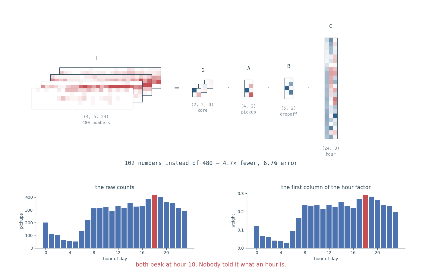
480 numbers become 102. The two charts are TODO 6. On the left, the busiest hour in the raw counts. On the right, the peak of the hour factor — which the decomposition built without ever being told what an hour is.
The result: 4.7× fewer numbers, 6.7% error. But the important part is TODO 6. The strongest pattern in the hour factor peaks at hour 18 — and that is also the busiest hour in the raw data. The decomposition found evening rush hour without being told what an hour is. That is expected rather than magic: every entry is a trip count, so the strongest pattern along the hour axis follows how busy each hour is. It found the dominant pattern along that axis, because that is what a decomposition does. The Tucker and CP stage runs this same decomposition live, on this same tensor, with the three ranks as sliders, so this table’s 480 → 102, 4.71× and 6.7% move under your own hand as you change them.
Look at the einsum strings: 'ijk,ia,jb,kc->abc' contracts three axes in one expression. That is why einsum came first.
Where this is used. In tech, Tucker and CP compress the large weight tensors inside neural networks so models run on phones instead of servers. In biotech, applied to data such as (genes × samples × conditions), they find structure ordinary PCA cannot reach, because PCA can only ever see two axes. For real projects use tensorly, which implements both properly — see References for the Kolda & Bader survey and the theorem (Eckart–Young) underneath both decompositions.
Kahoot Quiz 3 — Convolution & Tensor Decompositions (5 min)
Run this right after section 10, before section 11. Its six questions still cover convolution and correlation alongside Tucker and CP. Convolution became take-home 13 when factorizations moved into the day, and the questions have not been rewritten yet. Run it while the taxi-tensor rush-hour result is still on screen. Launch kahoot_quiz_3_convolution_decompositions.xlsx (6 questions, ~5 min), then go straight from the podium into section 11, which takes the same tensor to CP.
11 · Tensor Factorizations: Which One, and What It Costs (Block 7, 15 min)
Practise today: Compare CP and Tucker on the same tensor using parameter counts, reconstruction errors, and the budget gap.
Explore later: Study Tensor Train and t-SVD, investigate CP uniqueness, and compress neural-network layers.
Section 09 asked which factorization, and what does it cost one order down, on matrices. This section asks it of tensors, straight after section 10 has shown one answer. The notebook is 11 · Tensor factorizations.
A tensor decomposition is not only a compression technique. Each one makes a different assumption about which structure in the data should be kept, and that assumption — not the flop count — is what you choose between.
Four decompositions, four bargains
| Method | Main idea | Storage | Best fit |
|---|---|---|---|
| CP | Sum of rank-1 components | R(I + J + K) |
Individually interpretable components; uniqueness can matter |
| Tucker / HOSVD | One low-dimensional subspace per mode, plus a core | R₁R₂R₃ + IR₁ + JR₂ + KR₃ |
Different modes need different ranks |
| Tensor Train (TT) | Chain of small cores | ≈ O(N · I · r²) |
Very high-order tensors |
| t-SVD | FFT along mode 3, matrix SVDs, inverse FFT | Depends on retained tubal rank | Order-3 tensors with a meaningful third mode |
🇪🇸 Cada método conserva una estructura distinta. CP busca componentes individuales, Tucker permite un rango diferente por modo, Tensor Train evita que un núcleo de orden alto crezca exponencialmente, y t-SVD conserva la estructura del tercer modo mediante FFT.
Why not flatten first?
Flattening preserves the numerical entries but can hide the meaning carried by separate tensor modes. The synthetic fluorescence-unmixing example in the notebook makes the difference measurable:
- CP recovers the true component amounts at correlation
1.00. - Flatten-then-SVD reaches only mean
|corr| ≈ 0.536. - The SVD representation can produce negative amount directions, even though a physical concentration cannot be negative.
That example is synthetic by design: it isolates the structural question without requiring another dataset download.
🇪🇸 Aplanar no es necesariamente incorrecto. El problema aparece cuando fusionamos dos modos cuyo significado separado era precisamente la información que queríamos interpretar.
Fair comparison: CP versus Tucker
Do not compare CP rank R against Tucker rank (R, R, R). Those two representations store different numbers of parameters, so the comparison measures the budget, not the model. A fair experiment is:
- choose a CP rank;
- count its stored parameters,
R · sum(T.shape); - search Tucker ranks near that same parameter budget, and keep the one with the lowest reconstruction error;
- compare error and interpretability at that matched budget.
Step 3 is where this goes wrong most easily. Picking the candidate whose parameter count is merely closest to the budget can hand Tucker a degenerate rank-1 mode, and manufacture the conclusion. The notebook runs the comparison this way on the real NYC taxi tensor, pickup borough × dropoff borough × hour. It uses the workshop’s pinned storm clip as a second tensor-shaped example. The budget picture on the Tucker and CP stage draws exactly this: CP’s error against its parameter count for R = 1 through 6, a cloud of every Tucker rank triple that fits inside each budget, and a toggle between best error and closest params so you can watch the second rule hand Tucker a degenerate rank-1 axis on the same tensor this section is about.
# TODO 1: Choose a CP rank R for the taxi tensor.
# TODO 2: Count CP parameters: R * sum(T.shape).
# TODO 3: Search Tucker ranks near that parameter count and keep the one with
#         the lowest reconstruction error, not merely the closest parameter
#         count. Watch what a rank-1 mode does to the answer.
# TODO 4: Compare relative reconstruction error at the matched budget.
# TODO 5: Explain which set of factors is easier to interpret.
Why Tensor Train matters as order grows
For a dense order-N tensor with equal mode size I, dense storage is I^N. At a fixed TT bond rank r, TT storage is ≈ O(N · I · r²): exponential in the order against linear in the order, with I and r held fixed.
CP storage is also linear in the order under a fixed global rank. TT’s practical advantage is different: it represents high-order interactions through local bond ranks, rather than through one Tucker core that grows exponentially with the order.
# TODO 1: Fix I and the TT bond rank r.
# TODO 2: Increase the tensor order N.
# TODO 3: Plot dense storage I**N against TT storage ~ N*I*r**2.
# TODO 4: Explain the different growth rates, and where the crossover sits.
Tensor decomposition inside neural networks
A dense convolution kernel of shape 3 × 3 × 512 × 512 holds 2,359,296 weights, and costs about 462 million multiply-adds on a 14 × 14 feature map. A CP factorization at rank 64 stores 64 × (3 + 3 + 512 + 512) = 65,920 weights — 35.8× fewer — and runs as four skinny convolutions in sequence: 1×1 → 3×1 → 1×3 → 1×1.
One order up, a transformer output matrix W_O of shape 4096 × 4096 stores 16,777,216 weights; a TT-matrix representation at rank 16 stores 34,816, or 481.9× fewer.
The storage ratio is the easy half. The workflow that makes it usable is train → compress → fine-tune. Compression buys you nothing unless the downstream task stays accurate enough, and that is a property of the trained weights, not of the shape.
# TODO 1: Build the synthetic convolution kernel from notebook 13.
# TODO 2: Evaluate several CP ranks.
# TODO 3: Find the smallest rank whose reconstruction error sits below a
#         threshold you chose in advance.
# TODO 4: Report the rank, the error, the stored weights and the compression
#         ratio — all four, because any one of them alone can be gamed.
The decision rule
Choose the decomposition from the structure you need to preserve, then choose the rank from the loss you can afford. Keep that order. The first question has no numerical answer, and the second has no answer at all until the first is settled.
🇪🇸 Elige primero el método según la estructura que necesitas conservar. Después elige el rango según el error, el almacenamiento o el coste que puedes aceptar.
For the full interactive treatment — method chooser, measured timing, matched-budget CP/Tucker comparison, downstream compression and the storage-budget widget — continue with 11 · Tensor factorizations.
Still open: the rank of 3 × 3 matrix multiplication
Multiplying two 2 × 2 matrices the schoolbook way takes 8 multiplications. In 1969 Volker Strassen did it with 7. Applied to blocks, over and over, that one saved multiplication cuts the cost of an n × n product from n³ to n^2.807, because log₂ 7 = 2.807. Two years later Winograd proved that 7 is the fewest possible.
That 7 is a CP rank. Matrix multiplication is a contraction, as section 06 showed, and a fixed tensor of 0s and 1s says which products it adds up. For 2 × 2 matrices that tensor is 4 × 4 × 4, with one 1 for each of the 8 schoolbook products. Each rank-one term of a CP decomposition costs one multiplication, so a rank-R decomposition is an algorithm with R multiplications. Strassen’s algorithm is seven rank-one terms that add up to the tensor exactly. The code below builds the tensor, checks that contracting it multiplies, and checks Strassen’s seven terms:
import itertools

import numpy as np

def matmul_tensor(n):
    # One 1 for each schoolbook product A[i, k] * B[k, j], added into C[i, j].
    M = np.zeros((n * n, n * n, n * n), dtype=int)
    for i, j, k in itertools.product(range(n), repeat=3):
        M[i * n + k, k * n + j, i * n + j] = 1
    return M

M2, M3 = matmul_tensor(2), matmul_tensor(3)
print(M2.shape, M2.sum(), M3.shape, M3.sum())  # (4, 4, 4) 8 (9, 9, 9) 27

# Contract M3 with two flattened 3 x 3 matrices, and out comes their product.
rng = np.random.default_rng(0)
A, B = rng.random((3, 3)), rng.random((3, 3))
C = np.einsum("abc,a,b->c", M3, A.ravel(), B.ravel()).reshape(3, 3)
print(np.allclose(C, A @ B))  # True

# Strassen's seven products. Row r of U and of V says which entries of A and
# of B product r adds up before it multiplies; row r of W says which entries
# of C it is added to (1) or subtracted from (-1). Order: 11, 12, 21, 22.
U = np.array([[1, 0, 0, 1], [0, 0, 1, 1], [1, 0, 0, 0], [0, 0, 0, 1],
              [1, 1, 0, 0], [-1, 0, 1, 0], [0, 1, 0, -1]])
V = np.array([[1, 0, 0, 1], [1, 0, 0, 0], [0, 1, 0, -1], [-1, 0, 1, 0],
              [0, 0, 0, 1], [1, 1, 0, 0], [0, 0, 1, 1]])
W = np.array([[1, 0, 0, 1], [0, 0, 1, -1], [0, 1, 0, 1], [1, 0, 1, 0],
              [-1, 1, 0, 0], [0, 0, 0, 1], [1, 0, 0, 0]])
print(np.array_equal(np.einsum("ra,rb,rc->abc", U, V, W), M2))  # True: rank <= 7
For 3 × 3 matrices the tensor is 9 × 9 × 9, with 27 ones, and nobody knows its rank. It is at least 19 (Bläser, 2003) and at most 23 (Laderman, 1976). Rank 21 would beat Strassen: recursing on 3 × 3 blocks would cost n^2.771. Rank 22 would not, at n^2.814.
Why it is worth money. Dense matrix multiplication is the core operation in training and running a neural network, so a cheaper one matters to anyone paying for the hardware. DeepMind has searched for low-rank decompositions of these tensors twice, with AlphaTensor (2022) and AlphaEvolve (2025). By Tamara Kolda’s account, neither beat the best practical exponent known at the time, Smirnov’s from 2013. The exponent also counts multiplications only: a fast algorithm still has to win on additions, memory traffic and rounding error before a library will use it.
Kolda, co-author of the survey the references page tells you to start with, has put the 9 × 9 × 9 problem to audiences since at least 2015, and posed it again on 28 September 2026 as a test for AI: An Open Problem to Challenge AI Math Skills. Grey Ballard, her co-author, conjectures that the rank is 23, so what is missing may be a proof that nothing shorter exists. Her post lists the same 27 ones, counted from 1 and with the first two axes numbered column by column rather than row by row; renumbering an axis cannot change a rank. The papers behind every number in this note are under An open problem on the references page, with a catalogue of the best known decompositions for every small size.
🇪🇸 Nadie conoce el rango del tensor
9 × 9 × 9de 27 unos que codifica la multiplicación de matrices 3 × 3: está entre 19 y 23. Un rango 21 daría un algoritmo más rápido que el de Strassen.
12 · Wrap-Up (5 min)
Practise today: Transfer axis reasoning to new data and explain why Tucker restores shape while losing information.
Explore later: Choose take-home work on PCA, attention, CP, Cholesky, audio, or deep dives 13–16.
What you did today:
- Part I — read a real photograph as a tensor: shape
(512, 512, 3), 786,432 numbers, and an axis known by what it means as well as by its size. - Part II — shuffled a batch of digits and a clip of video with the same permutation: the digits kept their labels and the video lost its story, because a batch axis and a time axis are different kinds of axis.
- Part III — standardized 1,797 digits with broadcasting and hit the pixels that never vary and turn into NaN; moved the channel axis of real microscopy images and caught the one reshape that runs without an error and scrambles a photograph; and kept 16 of a real video’s 720 frames, each traced back to the frame it came from.
- Part IV — turned a colour image grey with one
einsum; watched the pseudoinverse pick the smallest of many equally good answers when two columns are copies of each other; ran Fibonacci as a matrix power; fitted real airline traffic by QR and by the normal equations, and found similar residuals hiding different coefficients; and shrank a real taxi tensor from 480 counts to 60 numbers with Tucker, keeping one daily pattern that peaks at hour 18, before CP won the same game once the error bar dropped to 2%.
One idea connects sections 07, 09 and 10: when a problem has no exact answer and no true inverse, you do not give up. You find the best stable approximation instead. Those three sections state it. You watch it happen three times: the pseudoinverse on two columns that are copies of each other in section 07, Tucker on the taxi tensor in section 10, and Richardson-Lucy on a blurred photograph in take-home 13.
Where to go next - torch.einsum / tf.einsum / jnp.einsum — identical syntax to what you used today. - np.linalg — the rest of Chapter 2: eigendecomposition, lstsq, pinv, qr, cholesky. - scipy.signal and skimage.restoration — convolution and deconvolution beyond today. - The five take-homes, Appendices A to E — PCA, attention, CP, Cholesky and audio denoising — all of them in notebook 12. - A deep dive beyond them: convolution and deconvolution (Appendix F, notebook 13) — the third instance of today’s connecting idea, and the one the room did not run. See the notebook index for all take-home deep dives. - An open problem at the end of section 11: a 9 × 9 × 9 tensor of 27 ones whose rank nobody knows, and why a cheaper matrix multiplication is worth finding. - References and further reading — books, the seminal Tucker/CP/SVD papers, tensorly and the blog posts, for going deeper than today’s 210 minutes.
Further Reading
The bibliography moved to its own page, in both languages: References and further reading.
It carries what this section used to: the linear algebra books, the Kolda & Bader survey, the Tucker, CP/PARAFAC and Eckart–Young papers with their DOIs and author pages, and the tensorly docs. It adds the ML blog posts the slides link, which were never listed here at all. Each work is cited in exactly one place now, and the Spanish half of the site can reach it.
Jump straight to a group: linear algebra · tensors · an open problem · software · the ML blog.
The machine-generated companion is a different kind of thing, and lives on its own page. It is generated, not written. Check it against the works on that page, not the other way round.
Appendix A — Take-Home: How Many Principal Components Are Enough?
Real data contains a trap here. Find it.
bc = load_breast_cancer(); X, y = bc.data, bc.target

# TODO 1: Center X, run np.linalg.svd, and compute the fraction of variance each
#         component explains (variance is proportional to S**2).
# TODO 2: How many components explain 95% of the variance? The answer will look
#         TOO GOOD. Do not trust it yet.
# TODO 3: Print X.var(axis=0). The 30 measurements use different units — some are
#         areas in the thousands, some are ratios below 1. What is that doing?
# TODO 4: Redo everything on standardized data: (X - mean) / std. How many now?
# TODO 5: Scatter-plot the first 2 components, coloured by y. Do the two groups separate?
Solution
Xc = X - X.mean(axis=0)
S = np.linalg.svd(Xc, full_matrices=False)[1]
n95 = np.argmax(np.cumsum(S**2/(S**2).sum()) >= 0.95) + 1      # 1  (!)

Xs = (X - X.mean(axis=0)) / X.std(axis=0)
S2 = np.linalg.svd(Xs, full_matrices=False)[1]
n95_scaled = np.argmax(np.cumsum(S2**2/(S2**2).sum()) >= 0.95) + 1 # 10worst area has a variance around 323,000 while smoothness values sit below 1, so PCA reports the largest unit, not the largest pattern. After standardizing, the first component explains 44% and 10 components are needed. PCA knows nothing about units. Features on different scales must be standardized first.
Appendix B — Take-Home: Attention Is Two Contractions
Attention answers question 5 from the video-pipeline discussion: which parts of a sequence matter most? Protein language models use it so every amino acid can look at every other one. Recommenders use it to weight a user’s past interactions.
np.random.seed(6)
batch, seq_len, dim = 4, 12, 16
Q, K, V = (np.random.randn(batch, seq_len, dim) for _ in range(3))

def softmax(x, axis=-1):
    x = x - x.max(axis=axis, keepdims=True)
    e = np.exp(x); return e / e.sum(axis=axis, keepdims=True)

# TODO 1: With einsum, compute scores[b,i,j] = how much position i attends to
#         position j. Shape (4, 12, 12). Scale by 1/sqrt(dim).
# TODO 2: Apply softmax on the correct axis so each row of weights sums to 1.
# TODO 3: With einsum, combine V using those weights -> (4, 12, 16).
# TODO 4: Suppose the last 3 positions are padding, not real data. Build a mask,
#         set those scores to -np.inf BEFORE the softmax, and verify the padded
#         positions receive exactly zero weight.
Try it first on the attention stage: the same two contractions, with a sequence of four small enough to add up by hand, the scores drawn as a heatmap and softmax’s causal mask giving exact zeros rather than small positive weights.
🇪🇸 Pruébalo primero en el escenario de atención: las mismas dos contracciones, con una secuencia de cuatro lo bastante pequeña para sumar a mano, las puntuaciones dibujadas como un mapa de calor y la máscara causal de softmax dando ceros exactos en vez de pesos positivos pequeños.
Solution
scores  = np.einsum('bid,bjd->bij', Q, K) / np.sqrt(dim)
weights = softmax(scores, axis=-1)
output  = np.einsum('bij,bjd->bid', weights, V)

mask = np.zeros((seq_len, seq_len)); mask[:, -3:] = -np.inf
weights_masked = softmax(scores + mask, axis=-1)     # padded positions get weight 0
scores is Chapter 2’s dot product (eq. 2.8); output is Chapter 2’s linear combination (eq. 2.28). Attention is two contractions built from ideas you have already read. TODO 4 solves the variable-length problem from Part II: the mask is how real models handle sequences and videos of different lengths.
Appendix C — Take-Home: CP vs Tucker
The CP-versus-Tucker exercise that lived here has moved into the session itself, as 11 · Tensor factorizations. There CP and Tucker are compared at a matched parameter budget rather than rank-for-rank, and the discussion extends to Tensor Train and t-SVD. Section 11 is the written companion to that notebook, and the Tucker and CP stage runs the whole comparison live in the browser, on the same taxi tensor, with no notebook to launch.
🇪🇸 El ejercicio de comparación entre CP y Tucker se trasladó al cuaderno 11 · Factorizaciones tensoriales, donde CP y Tucker se comparan con un presupuesto de parámetros equivalente, y el análisis se amplía a Tensor Train y t-SVD.
Appendix E — Take-Home: Audio Denoising by Low-Rank STFT
The truncated SVD is the optimal low-rank approximation (Eckart–Young, in the references). This appendix is where that optimality stops being enough. Cut a real voice recording into short overlapping time windows, and ask which frequencies are present in each. That is the short-time Fourier transform, and its output is a matrix, frequency × time. Truncating that matrix’s SVD keeps the structure concentrated in the leading singular directions and throws the rest away. If the voice is more concentrated there than the noise is, the result is cleaner. If it is not, you have thrown away the voice.
Each of those moves is a picture on the audio tensor stage, computed in the browser from this same recording. It cuts one window out of the array and shows the taper being applied to it; it asks that one window which frequencies are in it, drawing all 1024 bins with the mirror half greyed out, which is why the matrix below has 513 rows and not 1024; and it hops the window along so that each stop is one column of the (513, 465) you are about to factor. Play the rebuilt signal there with the overlap set to none and you can hear why the windows have to overlap. The truncation itself is the low rank picture: it adds the same 5 dB of noise, factors the matrix while you wait, and rebuilds this table’s curve point by point rather than quoting it.
Optimal on ‖A − B‖_F is not the same as optimal on the thing you care about, so the criterion has to be measured, not assumed. Here the criterion is signal-to-noise ratio against a known clean reference — which is why the noise is added deliberately rather than found. The recording is real and pinned to a SHA-256; the noise is synthetic by design, because only a known clean signal makes SNR measurable at all.
real voice → controlled noise → STFT matrix → SVD truncation → ISTFT → SNR
VOICE_URL = ("https://raw.githubusercontent.com/pdx-cs-sound/wavs/"
             "ed5ebcbbbc2d11f0adddc9b50b78d581c29f738c/voice.wav")
VOICE_SHA256 = "2c4b4d9d5f90715fdbf599869a465d521638f40ca978b186df96f1543a4d67dc"

def snr_db(reference, estimate):
    return 10 * np.log10(np.sum(reference**2)
                         / np.sum((estimate - reference)**2))

# TODO 1: Download voice.wav, check its SHA-256 before using it, and refuse the
#         file if it does not match. Convert to float and mix down to mono.
# TODO 2: Add Gaussian noise scaled to a target SNR of 5 dB, then measure the
#         SNR you actually got. It should come back at 5 dB — that is the check
#         that your scaling is right.
# TODO 3: Take signal.stft(noisy, fs=fs, nperseg=1024, noverlap=512) and run
#         np.linalg.svd on it. The matrix is COMPLEX; svd handles that.
# TODO 4: For k in [2, 5, 10, 20, 40, 80, full_rank], rebuild the rank-k STFT,
#         invert it with signal.istft, and measure the SNR against `clean`.
# TODO 5: Plot SNR against k. It is not monotonic. Find the best k, and say
#         what is happening at BOTH ends of the curve.
# TODO 6: Why does full rank return exactly the SNR of the noisy input?
Solution
f, t, Z = signal.stft(noisy, fs=fs, nperseg=1024, noverlap=512)
U, s, Vh = np.linalg.svd(Z, full_matrices=False)          # Z.shape (513, 465)

for k in [2, 5, 10, 20, 40, 80, len(s)]:
    Zk = (U[:, :k] * s[:k]) @ Vh[:k, :]
    _, rec = signal.istft(Zk, fs=fs, nperseg=1024, noverlap=512)
    n = min(len(clean), len(rec))
    print(k, snr_db(clean[:n], rec[:n]), np.sum(s[:k]**2) / np.sum(s**2))
4.949 seconds at 48 kHz gives a (513, 465) STFT, so full rank is 465. The noisy input measures 5.00 dB, as constructed:
| k | SNR | Retained energy | |
|---|---|---|---|
| 2 | 2.29 dB | 33.2% | worse than the noise we started from |
| 5 | 4.76 dB | 51.1% | still worse |
| 10 | 6.78 dB | 61.9% | |
| 20 | 8.48 dB | 70.1% | |
| 40 | 9.08 dB | 78.3% | best — +4.08 dB, at 8.6% of full rank |
| 80 | 7.68 dB | 87.1% | past the peak |
| 465 | 5.00 dB | 100% | exactly the noisy input again |
Both ends fail, for opposite reasons. At k = 2 the approximation is so aggressive that it discards voice along with noise, and lands below the noisy signal — a “denoiser” that made things worse. At full rank nothing is discarded at all: U Σ Vᵀ reconstructs Z exactly, ISTFT inverts STFT, and you get the noisy audio back, 5.00 dB, unchanged. The useful region is the middle, and the peak here retains 78% of the singular-value energy from 8.6% of the ranks — which is the same compression story as the taxi tensor in section 10, measured against a different criterion.
k = 40 to k = 80 retains more energy (87% against 78%) and produces worse audio, because the energy being added back is noise. Low rank does not mean clean; it means small. Whether it also means better is an empirical question. This is the one take-home where the answer is “only in a window, and you have to measure to find it”.
Appendix F — Take-Home: Convolution and Deconvolution
The theory
Convolution slides a small array (the kernel, or filter) across a larger one, multiplying and summing at each position. It is the operation at the heart of every convolutional neural network, and it is also how every blur, sharpen, and edge-detection filter works.
x = np.array([1., 2., 3., 4., 5.])
k = np.array([1., 0., -1.])

np.convolve(x, k, 'full')    # [ 1.  2.  2.  2.  2. -4. -5.]  length 5+3-1 = 7
np.convolve(x, k, 'valid')   # [ 2.  2.  2.]                  length 5-3+1 = 3
np.convolve(x, k, 'same')    # [ 2.  2.  2.  2. -4.]          length 5
Three modes, three output sizes. valid uses only positions where the kernel fits completely — this is why convolution shrinks an image by kernel_size - 1.
⚠️ A detail that catches almost every reader. True convolution flips the kernel. Correlation does not. What deep learning libraries call “convolution” is actually correlation. It makes no practical difference, because the network learns the kernel — but you should know the names are inconsistent.
np.correlate(x, k, 'valid')          # [-2. -2. -2.]
np.convolve(x, k[::-1], 'valid')     # [-2. -2. -2.] — the same, with k flipped
Convolution is a matrix multiplication. This is the connection back to Chapter 2. Any convolution can be written as multiplication by a Toeplitz matrix — a matrix where the kernel is shifted along each row:
col = np.zeros(7); col[:3] = k
row = np.zeros(5); row[0] = k[0]
C = toeplitz(col, row)                       # (7, 5)
np.allclose(C @ x, np.convolve(x, k, 'full'))   # True
So convolution is not a new kind of operation. It is a structured matrix multiplication, one where the same few numbers are reused at every position in the matrix. That reuse is exactly why CNNs need so many fewer parameters than fully connected networks.
Deconvolution means two different things, and you must keep them separate:
- Transposed convolution — the upsampling layer in a decoder or GAN. It makes things bigger. It is not a true inverse; the name is historical and misleading.
- True deconvolution — recovering the original signal from a blurred one. This is a genuine inverse problem, and it is where section 07 comes back.
Exercise (10 min)
img = data.camera().astype(float) / 255.      # real photograph, 512x512
sobel = np.array([[-1,0,1],[-2,0,2],[-1,0,1]], float)

# TODO 1: Convolve `img` with `sobel` in 'valid' mode. What shape comes out,
#         and by how much did it shrink?
# TODO 2: Blur the image with a 9x9 averaging kernel (all entries equal,
#         summing to 1), mode='same'. Display it next to the original.
# TODO 3 (transposed convolution): upsample this 2x2 array to 3x3 by adding
#         small * kernel into an output array at each position:
#             small = np.array([[1., 2.], [3., 4.]]); ker = np.ones((2, 2))
#         What shape do you get? Why is this called "deconvolution" in CNNs
#         even though it does not undo anything?
# TODO 4 (true deconvolution): add small noise to the blurred image, then try to
#         recover the original with skimage.restoration.richardson_lucy(...,
#         num_iter=50). Measure error BEFORE and AFTER, ignoring a 25-pixel
#         border. Did it improve?
Explanation (5 min)
edges = signal.convolve2d(img, sobel, mode='valid')     # (510, 510) — shrank by 2

psf = np.ones((9, 9)); psf /= psf.sum()
blurred = signal.convolve2d(img, psf, mode='same', boundary='symm')
noisy = blurred + 0.002 * np.random.default_rng(0).standard_normal(blurred.shape)

from skimage.restoration import richardson_lucy
recovered = richardson_lucy(np.clip(noisy, 0, 1), psf, num_iter=50)

c = 25   # ignore the border: deconvolution always creates edge artifacts
err = lambda a: np.linalg.norm((a-img)[c:-c,c:-c]) / np.linalg.norm(img[c:-c,c:-c])
print(err(noisy), err(recovered))     # 0.1157 -> 0.0815
Deconvolution reduced the error by about 30%. Two lessons worth keeping:
First, you must ignore the border. Deconvolution creates strong artifacts at the edges, where the algorithm has no information about what lies outside the image. If you measure error over the full image, border artifacts dominate and it looks like the method failed. It did not.
Second, why not just invert the blur directly? Because it fails badly. Blurring destroys high-frequency detail, so inverting it divides by numbers very close to zero and amplifies noise enormously:
K = np.fft.fft2(psf, s=img.shape)
naive = np.real(np.fft.ifft2(np.fft.fft2(noisy) / np.where(abs(K) < 1e-3, 1e-3, K)))
# relative error ≈ 1.4 — far WORSE than the blurred image we started from
This is the same lesson as section 07. A direct inverse either does not exist or is unusable, so you use a method that finds the best stable answer instead. The pseudoinverse does this for linear systems; Richardson-Lucy and Wiener filtering do it for deconvolution. In biotech this is routine. Every fluorescence microscope blurs its images by a known amount, the point spread function, and deconvolution is standard practice before cells are counted or measured.
Appendix G — Facilitator Notes
(Students may ignore this section.)
Structure. Four parts that build on each other: understand what a tensor is → reason about why axes exist → manipulate axes → compute with and factorize tensors. Sections 07, 09 and 10 share one theme: no exact inverse exists, so find the best stable approximation. Stating that connection out loud at the wrap-up is what makes the second half feel like one lesson rather than four.
Do not rush Part I. It is the students’ first contact with tensor theory and every later block uses its vocabulary. If running late, follow the Cutting for time order below.
Language. Students are ESL (Colombia). Speak slowly, avoid idiom, and define terms on first use. Name the Spanish cognates aloud early — eje, descomposición, contracción, convolución — it removes friction immediately. Invite questions in either language. Warn about the two meanings of “rank” at the start of Part I.
Verified numbers. Every output quoted in this document was executed and checked: malignant vs benign mean radius 17.5/12.1; 3 zero-variance digit pixels; 207 missing values in the housing data; housing RMSE ≈ 75,980; deconvolution error 0.1157 → 0.0815 (25-pixel border excluded); taxi Tucker 4.71× compression at 6.7% error with the hour factor peaking at 18; for Appendix E, a 4.949 s recording giving a (513, 465) STFT whose best tested rank is 40 at 9.08 dB against the noisy input’s 5.00 dB; and, for section 09, the degree-10 airline Vandermonde at κ(X) = 2.16e7 and κ(XᵀX) = 4.65e14, with coefficient errors of 1.95e-03 by the normal equations against 2.04e-14 by QR, and rank 16 of the astronaut image at 21.1 dB. If a student gets something different, it is worth investigating rather than dismissing. The one exception is section 09’s timings. Those are properties of the machine, not of the data. A Colab CPU will not reproduce them, which is why the appendix quotes ratios rather than milliseconds.
The downloads. Three CSVs from GitHub raw URLs, and the storm clip from Wikimedia for sections 02 and 05. Each notebook retries a download and then falls back to the workshop’s own copy on this site (data/), so a host that is down costs a few seconds, not a section. Even so, confirm in the first 5 minutes that notebook 00’s setup printed its shapes: a student who gets the bilingual “could not download” message has no network at all, and should pair with a neighbour.
Pre-assign the breakout groups for the video-pipeline block before the session; assigning them live costs 3–5 minutes.
The group block needs firmer facilitation than exercise blocks. If a group is still on the first design question with 5 minutes left, join their channel and tell them to sketch a shape, even the wrong one. The share-back matters more than a correct sketch.
The three Kahoot quizzes. Each is 6 questions in kahoot_quiz_1_vocabulary_shapes.xlsx, kahoot_quiz_2_distance_pseudoinverse.xlsx, and kahoot_quiz_3_convolution_decompositions.xlsx, sitting after sections 04, 07 and 10 respectively. Import each into a kahoot ahead of time (Create → Add question → Import → Import spreadsheet) — don’t do this live. Budget 5 minutes per quiz including the podium; groups tend to want to see the leaderboard, and that’s fine, it’s the payoff. These add 15 minutes total, taking the workshop from 195 to 210 minutes.
Cutting for time. In order: drop Kahoot Quiz 2 (the least novel of the three — the pseudoinverse comes back on the wrap-up’s one-idea slide), then Kahoot Quiz 1. Everything past a notebook’s Core complete, and every appendix, already sits outside the 210 minutes, so cutting it saves nothing. Never cut Part I §1.3, section 10, or Kahoot Quiz 3 — the last one checks whether Tucker landed while the taxi result is still on screen. The facilitator run sheet’s If you are behind turns this into clock-time checkpoints with a cut for each.
Known rough edges. Appendix F TODO 4 is the hardest thing in the workshop. A student who skips the border crop will conclude deconvolution failed, so flag the 25-pixel crop clearly before the exercise starts, not after. Section 07 TODO 3 asks students to trigger an error deliberately — some will think they did something wrong, so say in advance that the error is the expected result.