Text as Data

Day 1 · Foundations Module 1 95 minutes (45 briefing, 50 lab) 09:10 briefing · 09:55 lab

Tokenization, n-gram language models, TF-IDF and linear classifiers: the count-based baseline everything else is measured against.

Open the lab in Colab NumPy scikit-learn

Duration: 95 minutes (45 briefing, 50 lab)
Level: 200 · Intermediate
Lab runtime: Google Colab, CPU runtime · about 2 minutes of compute
Accounts and cost: Google. Free
Without API keys: the lab always runs its real models

What You Will Build

In this module you will:

Tokenize text and justify the choices
Build and evaluate an n-gram language model
Train a linear text classifier and read its errors

New terms, in the glossary: token, vocabulary, n-gram model, smoothing, cross-entropy, perplexity, logit, softmax, checkpoint cell.

Before You Start

Setup and Environment Check: the 10-minute notebook that checks your Colab runtime and loads any keys.
A Google account. Colab’s default CPU runtime is enough.
No API keys: the lab runs its own models throughout.

Where we start. You can already fit a logistic regression to a table of numbers and read its loss. What you have not done yet is turn a string into those numbers. The five days run from counting words (today) to learned vectors and attention, then to transformers and pretrained models (Day 2), to using those models through APIs and what they are trained to prefer (Day 3), to how far their confidence can be trusted and how to ground their answers in sources (Day 4), and to agents and systems built out of them (Day 5). This module asks one question: how far does counting alone get us, and where exactly does it stop?

In the Lab

Open the lab in Colab

6 exercises in 2 parts. The notebook budgets 50 minutes for them; the lab slot is 50 minutes. Each exercise you write is a # TODO stub with a folded solution beneath it and a checkpoint that passes or fails; where people tend to stall, a folded hint sits above the stub.

Task	Briefing section	Time
Part A · Language Modeling by Counting
Exercise 1 · Tokens and Vocabulary	2	8 min
Exercise 2 · Counting N-Grams and Add-k Smoothing	3	12 min
Exercise 3 · Perplexity	3	8 min
Exercise 4 · Sampling	3	5 min
Part B · Text Classification by Counting
Exercise 5 · TF-IDF and Two Linear Classifiers	4, 5	10 min
Exercise 6 · Precision, Recall, F1 and Reading the Errors	6 (Reference)	7 min

Challenge · BM25

Optional, for anyone who finishes the core path early: the notebook’s stretch section, after the last checkpoint.

When you are done. Runtime → Disconnect and delete runtime releases the machine; your keys stay in Colab Secrets for the next lab.

Agenda

Minutes	Section	In the room
0–5	1. What Makes Language Hard	—
5–14	2. Tokens, Vocabularies and Zipf’s Law	Check yourself (2 min)
14–30	3. N-Gram Language Models	Demo (4 min)
30–35	4. Bag-of-Words and TF-IDF	—
35–40	5. Naive Bayes and Logistic Regression	—
40–45	7. Where Count-Based Methods Stop Working	Check yourself (2 min)
45	Total	37 minutes of exposition, 8 of activities

Checks, demos and predictions listed here are part of the live session and its minutes; the others on the page are for reading afterwards.

Read now · Sections 1–5 and 7, in the agenda above.

Use in the lab · Exercise 1: section 2; Exercises 2–4: section 3; Exercise 5: sections 4 and 5; Exercise 6: section 6 (section 6: Reference; the exercise restates what it needs).

Read later · Section 6, Evaluation: Precision, Recall and F1 (Reference); the collapsed callouts marked Optional or After the Lab; Further Reading.

Notation

Notation used on every module page: a text is a sequence of tokens w_1, \dots, w_T of length T; the vocabulary is V, with size |V|; c(\cdot) is a count in the training data; x is an input vector, y a label, C the number of classes; \theta are parameters and \mathcal{L} is a loss. All logarithms are natural.

1. What Makes Language Hard

Objective: name the three properties of language that every model in this workshop has to deal with.

A model needs numbers. Text is a string of symbols. This module covers the simplest way across that gap: count things. Before we do, it helps to know why the gap is wide.

Ambiguity. One string, several meanings.

I saw her duck. A bird she owns, or a movement she made?
She ate the pizza with a fork and she ate the pizza with anchovies have the same word-class pattern, but “with a fork” modifies the eating and “with anchovies” modifies the pizza.

People resolve these with context and world knowledge, usually without noticing. A model has to learn to do the same from data.

Sparsity. Most things you could say have never been said. With a vocabulary of |V| = 10^4 words there are 10^{12} possible three-word sequences. A training corpus of a million tokens contains at most 10^6 of them. So almost every legal three-word sequence has a count of zero, and a model that trusts raw counts will call it impossible.

Compositionality. The meaning of a sentence depends on its words and on how they are arranged. Dog bites man and man bites dog use the same words. A representation that throws away order cannot tell them apart.

Keep these three in view. Each later module is a response to one of them: word vectors (Module 2) to sparsity, sequence models and attention (Modules 3 to 5) to compositionality, and large-scale pretraining (Module 6) to the amount of context needed to resolve ambiguity.

Check yourself. Keep |V| = 10^4 and the corpus of 10^6 tokens. What is the largest share of the possible two-word sequences that the corpus can contain? Does shortening the sequence from three words to two remove the sparsity problem?

Answer

There are |V|^2 = 10^8 possible pairs, and a corpus of 10^6 tokens contains at most 10^6 distinct ones: at most 1%. So at least 99% of the pairs still have a count of zero. Each word removed from the sequence divides the number of possibilities by |V|, which helps, but it does not remove the problem, and it is paid for in context: a model that looks at one previous word knows less about what comes next.

2. Tokens, Vocabularies and Zipf’s Law

Objective: turn a string into a sequence of integer IDs, and say what each design choice costs.

Tokenization and Normalization

A tokenizer splits a string into units called tokens. Normalization maps variants of a string to one form before or after splitting (for example, lowercasing). The vocabulary V is the set of distinct tokens the model knows; each token gets an integer ID from 0 to |V| - 1.

The choices, and what each one trades:

Choice	Options	Trade-off
Unit	characters, words, subwords	Characters: tiny vocabulary, long sequences, nothing is ever unknown. Words: meaningful units, large vocabulary, unknown words at test time. Subwords (Module 6) sit between the two.
Case	keep, or lowercase	Lowercasing merges The and the (good) and US and us (bad).
Punctuation	separate token, attached, or dropped	Dropping it loses sentence boundaries and the difference between Let’s eat, Grandma and Let’s eat Grandma.
Rare words	keep all, or map to one unknown token	Keeping all makes the vocabulary huge and the counts unreliable. Mapping loses information.

There is no correct answer, only a choice that fits the task. A topic classifier loses little from lowercasing. A language model that must generate readable text needs case and punctuation.

Word-level models need a rule for words they have not seen. The standard one: replace every training word with count below a threshold by a special token <unk> (unknown), and do the same to any unseen word at test time. <unk> then has a count like any other token.

A word-level tokenizer in one line, as used in the lab:

import re

def tokenize(text):
    # runs of letters, digits or apostrophes, or any single non-space symbol
    return re.findall(r"[a-z0-9']+|[^a-z0-9'\s]", text.lower())

Lab 1, Exercise 1 asks you to write tokenize and build_vocab. A provided cell then measures how much of the held-out text the vocabulary covers; the measured coverage is in the box after the lab at the end of this section.

Check yourself. Apply tokenize by hand to the string The U.S. isn't us. How many tokens come out, and how many distinct vocabulary entries? Which information did the tokenizer keep, and which did it destroy?

Answer

Eight tokens: the, u, ., s, ., isn't, us, ., of which six are distinct (the period occurs three times). The apostrophe is inside the character class, so isn't stays whole. A period is not, so the abbreviation is split into u . s ., and its periods are now the same token as the one that ends the sentence. A model reading these IDs can no longer tell an abbreviation from a sentence boundary. That is a cost of this tokenizer, accepted because the lab’s tasks do not depend on it.

Zipf’s Law

Sort the vocabulary by frequency. Let r be the rank of a word (1 for the most frequent) and f(r) its count. Zipf’s law is the empirical observation that

f(r) \approx \frac{A}{r^{s}}, \qquad s \approx 1, \tag{1}

where A is a constant that depends on the corpus size and s is the exponent. Taking logs gives \log f(r) \approx \log A - s \log r: a straight line with slope -s on a log–log plot.

What this means in practice:

A few words (the, and, to) account for a large share of all tokens. In the lab corpus the ten most frequent words are 19% of all word tokens.
The curve has a long tail: a large share of the vocabulary appears once or twice. In many corpora roughly half of the distinct words appear exactly once.
Adding more data does not remove the tail. New rare words keep arriving.

So any estimate that depends on the count of a specific word, or worse, a specific word sequence, is unreliable for most of the vocabulary. That is the sparsity problem of Section 1 in quantitative form. Exercise 1 plots this curve for the lab corpus; the recorded plot is in the box after the lab, below.

After the Lab: What Lab 1 Measured in Exercise 1

Open this after Exercise 1, so that it does not answer the lab’s prediction for you. On the Shakespeare training split, keeping every word gives 11,908 entries and covers 96.1% of validation tokens; dropping words seen once (min_count = 2) nearly halves the vocabulary, to 6,463 entries, and still covers 94.0%. In the lab corpus 46% of the distinct words occur exactly once (Figure 1).

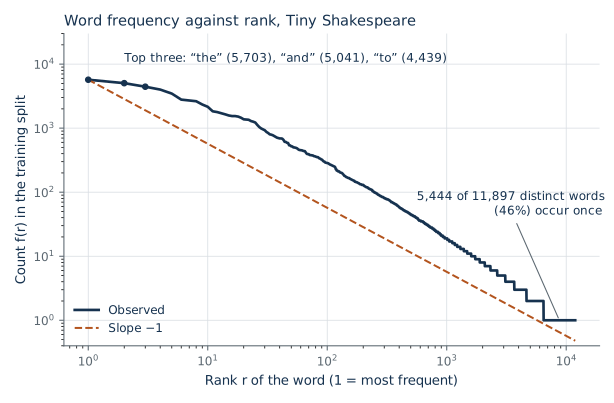
Log-log plot of word count against rank for Tiny Shakespeare. The observed curve falls roughly along a dashed reference line of slope minus one. The top three words are annotated: the (5,703), and (5,041), to (4,439). A label on the flat tail at count 1 reads: 5,444 of 11,897 distinct words (46 percent) occur once. — Figure 1: Word frequency against rank in the training split of the Shakespeare corpus, on log–log axes, with a reference line of slope -1. Punctuation tokens are left out. Measured with the Lab 1 tokenizer.

Check yourself. In the lab corpus the most frequent word, the, occurs 5,703 times. If Equation 1 held exactly with s = 1, about how often would the word of rank 100 occur? The word of rank 1,000? What does the second number mean for a bigram model that must estimate what follows that word?

Answer

Rank 1 gives A = f(1) = 5{,}703, so f(100) \approx 5{,}703 / 100 \approx 57 and f(1{,}000) \approx 5{,}703 / 1{,}000 \approx 6. A word seen six times has at most six observed continuations, out of roughly 12,000 possible next words. Its next-word distribution is estimated from six draws, and almost every entry is zero. Most of the vocabulary sits at rank 1,000 or beyond, so this is the normal case, not the exception. (The measured curve only roughly follows the line, so treat 57 and 6 as orders of magnitude.)

3. N-Gram Language Models

Objective: define a language model, estimate one from counts, fix its zeros, and measure it.

What a Language Model Is

A language model assigns a probability to a sequence of tokens. By the chain rule of probability, with no approximation,

P(w_1, \dots, w_T) = \prod_{t=1}^{T} P(w_t \mid w_{<t}), \tag{2}

where w_{<t} is shorthand for w_1, \dots, w_{t-1}, the tokens before position t. So modeling text reduces to one question, asked repeatedly: given what came before, what comes next? Every language model in this workshop, up to GPT, answers this same question. They differ only in how they compute P(w_t \mid w_{<t}).

The Markov Assumption

We cannot estimate P(w_t \mid w_{<t}) by counting: a long history w_{<t} almost never occurs twice. An n-gram model assumes that only the previous n - 1 tokens matter:

P(w_t \mid w_{<t}) \approx P(w_t \mid w_{t-n+1}, \dots, w_{t-1}). \tag{3}

Here n is the order of the model. With n = 2 (a bigram model) the context is one token; with n = 3 (a trigram model) it is two. We write the context as w_{t-n+1:t-1}. The first positions of a text are padded with n - 1 copies of a start token <s> so that every position has a full context.

Estimation by Counting

Let c(w_{t-n+1:t}) be the number of times the full n-gram occurs in the training data, and c(w_{t-n+1:t-1}) the number of times its context occurs. The maximum-likelihood estimate (MLE), the one that makes the training data most probable, is the relative frequency:

P_{\text{MLE}}(w_t \mid w_{t-n+1:t-1}) = \frac{c(w_{t-n+1:t})}{c(w_{t-n+1:t-1})}. \tag{4}

For a bigram model: of all the times we saw the, what fraction were followed by king?

The model is two tables of counts: one for full n-grams, one for contexts. In code, over a list of integer IDs, with bos the ID of <s>:

from collections import Counter

def ngram_counts(ids, n, bos):
    grams, contexts = Counter(), Counter()
    padded = [bos] * (n - 1) + list(ids)
    for t in range(n - 1, len(padded)):
        context = tuple(padded[t - n + 1 : t])   # the n - 1 IDs before position t
        grams[context + (padded[t],)] += 1       # c(w_{t-n+1:t})
        contexts[context] += 1                   # c(w_{t-n+1:t-1})
    return grams, contexts

Lab 1, Exercise 2 asks you to write ngram_counts: the numerator and denominator of Equation 4.

Optional: Why Relative Frequency Is the Maximum-Likelihood Estimate

Fix one context and let p_w be the probability of next token w, with c_w its count after that context. The log-likelihood of the training data for this context is \sum_w c_w \log p_w, to be maximized subject to \sum_w p_w = 1. Add a Lagrange multiplier \lambda for the constraint and set the derivative with respect to p_w to zero:

\frac{\partial}{\partial p_w}\Bigl[\sum_{w'} c_{w'} \log p_{w'} - \lambda \bigl(\textstyle\sum_{w'} p_{w'} - 1\bigr)\Bigr] = \frac{c_w}{p_w} - \lambda = 0 \quad\Rightarrow\quad p_w = \frac{c_w}{\lambda}.

Summing over w and using the constraint gives \lambda = \sum_w c_w, so p_w = c_w / \sum_{w'} c_{w'}.

The Zero Problem and Add-k Smoothing

Equation 4 gives probability zero to any n-gram that did not occur in training. Section 1 showed that this is most of them. One zero in the product Equation 2 makes the whole text impossible.

Smoothing moves some probability from seen n-grams to unseen ones. The simplest method, add-k smoothing, pretends every possible next token was seen k extra times after every context, where k > 0 is a constant we choose:

P_{\text{add-}k}(w_t \mid w_{t-n+1:t-1}) = \frac{c(w_{t-n+1:t}) + k}{c(w_{t-n+1:t-1}) + k\,|V|}. \tag{5}

The denominator follows from the numerator. We added k to each of |V| possible next tokens, so the context total rises by k|V|, and the probabilities still sum to one:

\sum_{w \in V} \frac{c(\text{context}, w) + k}{c(\text{context}) + k|V|} = \frac{c(\text{context}) + k|V|}{c(\text{context}) + k|V|} = 1.

Two things to notice:

A context never seen in training has c = 0 everywhere, so Equation 5 returns 1 / |V|: the uniform distribution. That is a sensible answer to “I know nothing”.
k is a hyperparameter: a setting chosen by us, not learned from the training data. Large k flattens every distribution toward uniform; small k trusts the counts. We choose it on a validation split, never on the test split. k = 1 is called Laplace smoothing and is usually too large for language models.

In this briefing k always means this smoothing constant. (From Module 4 on, k_i with a subscript denotes an attention key; the two never appear together.)

Lab 1, Exercise 2 implements Equation 5 as prob(w, context, counts, k, vocab_size); its checkpoint is the sum-to-one identity above. A provided cell after Exercise 3 shows the zero problem directly: with k = 0, 20.2% of the validation tokens get probability zero under a word-level bigram model.

Worked example: a bigram model on nine tokens. The training text, read as one stream, is the cat sat the dog sat the cat ran. The vocabulary is {the, cat, dog, sat, ran}, so |V| = 5. Take the context the. It occurs three times and is followed by cat twice and by dog once, so c(\textit{the}) = 3, c(\textit{the}, \textit{cat}) = 2 and c(\textit{the}, \textit{dog}) = 1.

Next token w	c(\textit{the}, w)	MLE (Equation 4)	Add-k with k = 0.5 (Equation 5)
cat	2	2/3 = 0.667	2.5 / 5.5 = 0.455
dog	1	1/3 = 0.333	1.5 / 5.5 = 0.273
sat, ran, the (each)	0	0	0.5 / 5.5 = 0.091

The add-k denominator is c(\textit{the}) + k|V| = 3 + 0.5 \times 5 = 5.5. The three unseen tokens now hold 3 \times 0.091 = 0.273 of the probability between them, all of it taken from cat and dog, and the column still sums to one: (2.5 + 1.5 + 3 \times 0.5) / 5.5 = 1.

Now take the context ran. It is the last training token, so nothing ever followed it and every count is zero. Equation 5 gives each token 0.5 / (0 + 2.5) = 0.2 = 1/|V|: the uniform distribution.

Check yourself. A context occurs three times in training and was followed by the same word every time. The vocabulary has |V| = 10{,}000 words. What probability does add-k give that word with k = 1 (Laplace)? With k = 0.01?

Answer

With k = 1: (3 + 1) / (3 + 10{,}000) \approx 0.0004. With k = 0.01: (3 + 0.01) / (3 + 100) \approx 0.029. Under Laplace smoothing, 99.96% of the probability goes to words that never followed this context, although every observation pointed to one word. By Zipf’s law most contexts are this rare, so this is the typical case. That is why k = 1 is usually too large for language models, and why k is chosen on validation data and not by convention.

Optional: Better Smoothing (interpolation, backoff, Kneser–Ney)

Add-k gives every unseen n-gram the same share. A better idea uses lower-order evidence: if the trigram drank green tea is unseen, the bigram green tea is still informative. Interpolation mixes orders with weights \lambda_1 + \lambda_2 + \lambda_3 = 1:

P(w_t \mid w_{t-2}, w_{t-1}) = \lambda_3 P_{\text{MLE}}(w_t \mid w_{t-2}, w_{t-1}) + \lambda_2 P_{\text{MLE}}(w_t \mid w_{t-1}) + \lambda_1 P_{\text{MLE}}(w_t).

Backoff uses the highest order that has a nonzero count. Kneser–Ney smoothing subtracts a fixed discount from every seen count and distributes it according to how many different contexts a word completes; it was the strongest count-based method for two decades (Chen and Goodman, 1999, in the readings). We do not need it here. The neural models of Modules 2 and 3 solve the same problem differently.

Perplexity

To compare language models we ask how well each predicts text it has not seen. Take a held-out sequence w_1, \dots, w_T. The average negative log-probability per token is the cross-entropy of the model on that text (in nats, because we use natural logs). Perplexity is its exponential:

\mathrm{PPL} = \exp\Bigl(-\frac{1}{T}\sum_{t=1}^{T} \log P(w_t \mid w_{<t})\Bigr). \tag{6}

Lower is better. How to read the number:

It is an effective branching factor. A model that spreads probability uniformly over the vocabulary has P = 1/|V| at every step, so \mathrm{PPL} = \exp(\log |V|) = |V|. A perplexity of 20 means the model is, on average, as uncertain as if it were choosing uniformly among 20 tokens.
It is the same quantity as the training loss of a neural language model. The cross-entropy loss printed by the LSTM in Module 3 and the transformer in Module 5 is \log \mathrm{PPL}. That is why this lab’s character-level number is directly comparable with theirs: all three average over the same characters of the same test split. A word-level perplexity is not (Module 3, section 6).
One zero makes it infinite. \log 0 = -\infty. An unsmoothed model has infinite perplexity on almost any held-out text.

import math

def perplexity(ids, history, n, counts, k, vocab_size):
    padded = list(history) + list(ids)           # history: the n - 1 IDs before ids
    total = 0.0
    for t in range(n - 1, len(padded)):          # exactly T = len(ids) predictions
        context = tuple(padded[t - n + 1 : t])
        total -= math.log(prob(padded[t], context, counts, k, vocab_size))
    return math.exp(total / len(ids))

One detail matters for comparisons. The training, validation and test splits are consecutive pieces of one text, so the first tokens of the validation split have real context: the end of the training split. history supplies those n - 1 tokens. They are context only, never predicted, and the average runs over the T tokens of the split. Only the very start of the training text is padded with <s>.

Lab 1, Exercise 3 implements Equation 6 and checks it against the uniform model.

Worked example, continued: perplexity. Score the held-out text the cat sat with the nine-token bigram model above and k = 0.5. The held-out text follows the training text, so the history is the last training token, ran. There are T = 3 predictions:

Prediction	Counts	Probability
P(\textit{the} \mid \textit{ran})	context never seen	0.5 / 2.5 = 0.200
P(\textit{cat} \mid \textit{the})	c(\textit{the}, \textit{cat}) = 2, c(\textit{the}) = 3	2.5 / 5.5 = 0.455
P(\textit{sat} \mid \textit{cat})	c(\textit{cat}, \textit{sat}) = 1, c(\textit{cat}) = 2	1.5 / 4.5 = 0.333

The cross-entropy is -\tfrac{1}{3}(\log 0.200 + \log 0.455 + \log 0.333) = 1.166 nats per token, and Equation 6 gives \mathrm{PPL} = e^{1.166} = 3.21. The uniform model over five tokens would score 5. On this text the counts are worth a reduction from five equally likely choices to about three.

Perplexities are comparable only when the two models predict the same tokens of the same text with the same vocabulary. A character-level perplexity and a word-level perplexity are different quantities. Mapping more words to <unk> lowers word-level perplexity without making the model better. In this workshop the number carried forward to Modules 3 and 5 is the character-level perplexity on the test split of the Shakespeare corpus.

Check yourself. With the same nine-token model and k = 0.5, score the held-out text the dog ran instead (history ran again). Is the model better or worse than uniform on this text? What happens with k = 0?

Answer

The three probabilities are P(\textit{the} \mid \textit{ran}) = 0.200, P(\textit{dog} \mid \textit{the}) = 1.5 / 5.5 = 0.273 and P(\textit{ran} \mid \textit{dog}) = 0.5 / (1 + 2.5) = 0.143, because dog ran never occurred. The perplexity is \exp\bigl(-\tfrac13(\log 0.200 + \log 0.273 + \log 0.143)\bigr) = 5.04, slightly worse than the uniform model’s 5: one unseen bigram cost more than the seen one gained. With k = 0 the third probability is 0/1 = 0, so the perplexity is infinite, and the first is 0/0: the unsmoothed estimate is not even defined after a context that was never seen.

Try it: how much to smooth. A word-level bigram model is trained on 20 tokens (the cat sat on the mat . the dog sat on the rug . the cat saw the dog ., |V| = 9) and scored on 13 held-out tokens (the dog saw the cat . the cat sat on the rug .). Two of the held-out bigrams, dog saw and cat ., never occur in training.

Predict first. As k grows from 0.001 to 10, does the held-out perplexity fall, rise, or do both? What value does it approach at the right-hand end?

viewof k = Inputs.range([0.001, 10], {value: 0.5, step: 0.001, transform: Math.log, label: "Smoothing constant k"})
viewof context = Inputs.select(["the", "cat", "dog", "sat", "mat"], {value: "the", label: "Context word"})

toy = {
  const train = "the cat sat on the mat . the dog sat on the rug . the cat saw the dog .".split(" ");
  const held = "the dog saw the cat . the cat sat on the rug .".split(" ");
  const vocab = [...new Set(train)];
  const grams = new Map(), contexts = new Map();
  const add = (m, key) => m.set(key, (m.get(key) ?? 0) + 1);
  for (let t = 1; t < train.length; t++) {
    add(grams, train[t - 1] + " " + train[t]);     // c(context, w)
    add(contexts, train[t - 1]);                   // c(context)
  }
  const count = (c, w) => grams.get(c + " " + w) ?? 0;
  const prob = (w, c, k) => (count(c, w) + k) / ((contexts.get(c) ?? 0) + k * vocab.length);  // add-k
  const ppl = (k) => {
    let total = 0, prev = train[train.length - 1];  // history: the last training token
    for (const w of held) { total -= Math.log(prob(w, prev, k)); prev = w; }
    return Math.exp(total / held.length);
  };
  return {vocab, count, prob, ppl};
}

{
  const V = toy.vocab.length;
  const rows = toy.vocab.map((w) => ({w, p: toy.prob(w, context, k), kind: toy.count(context, w) > 0 ? "seen after this context" : "never seen after it"}));
  const unseen = rows.filter((d) => d.kind !== "seen after this context").reduce((a, d) => a + d.p, 0);
  const curve = Array.from({length: 81}, (_, i) => 10 ** (-3 + i / 20)).map((kk) => ({k: kk, ppl: toy.ppl(kk)}));
  const bars = Plot.plot({
    width: 360, height: 240, marginBottom: 40,
    x: {label: "next token w", domain: toy.vocab}, y: {label: "P(w | context)", domain: [0, 1]},
    color: {legend: true, domain: ["seen after this context", "never seen after it"], range: ["var(--demo-blue)", "var(--demo-faint)"]},
    marks: [Plot.barY(rows, {x: "w", y: "p", fill: "kind"}), Plot.ruleY([1 / V], {strokeDasharray: "4 3"}), Plot.ruleY([0])]
  });
  const line = Plot.plot({
    width: 360, height: 240, marginBottom: 40,
    x: {type: "log", label: "k", ticks: [0.001, 0.01, 0.1, 1, 10], tickFormat: (d) => String(d)}, y: {label: "held-out perplexity", domain: [0, 10]},
    marks: [
      Plot.ruleY([V], {strokeDasharray: "4 3"}),
      Plot.text([{k: 0.0012, ppl: V}], {x: "k", y: "ppl", text: () => "uniform: |V| = 9", dy: -8, textAnchor: "start"}),
      Plot.line(curve, {x: "k", y: "ppl", stroke: "var(--demo-blue)", strokeWidth: 2}),
      Plot.dot([{k, ppl: toy.ppl(k)}], {x: "k", y: "ppl", r: 6, fill: "var(--demo-orange)"})
    ]
  });
  return html`<div style="display:flex;flex-wrap:wrap;gap:1.5rem;align-items:flex-end">${bars}${line}</div>
  <p>At k = ${k.toPrecision(3)}: tokens never seen after <em>${context}</em> hold ${(100 * unseen).toFixed(1)}% of the probability; held-out perplexity is ${toy.ppl(k).toFixed(2)}.</p>`;
}

The bar chart is the add-k distribution of Equation 5 after the chosen context; the dashed line is the uniform value 1/|V|. The curve is the held-out perplexity of Equation 6 as a function of k, with a dot at the current setting. It is a U. With very small k the two unseen bigrams get almost no probability and dominate the average. With large k every distribution flattens toward uniform and the perplexity climbs toward |V| = 9. The best k lies between, and you find it by measuring on held-out text, which is what the lab’s validation split is for.

Sampling

A language model is also a generator. Start from a context, draw the next token from P(\cdot \mid \text{context}), append it, slide the context window forward, repeat. Lab 1, Exercise 4 does this: you write the one line of sample that draws the next token, then compare samples from models of different order.

Raising n further exposes the weakness of add-k. Most long contexts were seen only once or twice, so their counts are small, and the k added to each of the |V| possible next tokens takes a large share of the probability. What that does to the samples is the lab’s prediction for Exercise 4; the box after the lab explains it.

After the Lab: What Lab 1 Measured in Exercise 4

Open this after Exercise 4, so that it does not answer the lab’s prediction for you. Character bigram samples are locally plausible and globally incoherent; at n = 3 fragments of English and the layout of a play appear. With the k that predicts held-out text best, high-order samples dissolve into random characters; with a much smaller k they copy the training text. At n = 5 with k = 0.01, a context seen once has total 1 + 0.01 \times 65 = 1.65, so about 39% of the probability goes to the 64 characters that never followed it. One such draw produces a context never seen in training, where Equation 5 is uniform, and the sample dissolves into random characters. With a much smaller k the same model stays fluent, but then its samples copy the training text more and more closely, because a context seen once has only one recorded continuation. The k that predicts held-out text best (the one chosen on validation) is not the one that generates the best-looking text.

Figure 2 measures that sparsity at the word level.

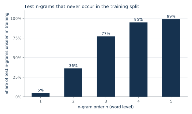
Figure 2: Share of word n-grams in the test split of the Shakespeare corpus that never occur in the training split, for n = 1 to 5. Raw words, no <unk> mapping. Measured with the Lab 1 tokenizer.

At n = 3, 77% of the test trigrams never occur in training. That is why, in the lab, the word-level trigram model has a higher test perplexity than the bigram model (1,437 against 304).

Check yourself. A colleague raises the <unk> threshold so that more rare words map to <unk>, retrains the word-level bigram model, and reports a test perplexity well below 304. Is the new model better? Push the threshold to its extreme to decide.

Answer

You cannot tell from the two numbers, because they are not comparable: the models predict different token sequences over different vocabularies. Predicting <unk> is easy, since it is now one of the most frequent tokens. At the extreme, every word is <unk>, the model predicts it with probability close to 1, and the perplexity approaches 1, the best possible value, for a model that says nothing about the text. Perplexity can only compare models that predict the same tokens of the same text with the same vocabulary.

4. Bag-of-Words and TF-IDF

Objective: represent a whole document as one vector.

We now switch tasks. In text classification the input is a document and the output is one of C labels. The running example is the topic-classification set: the title and abstract of an arXiv paper, labeled with one of C = 4 subject areas (language, vision, machine learning, robotics).

A classifier needs a fixed-length input x. The bag-of-words representation gives one dimension per vocabulary entry and stores a count:

x \in \mathbb{R}^{|V|}, \qquad x_w = c(w, D), \tag{7}

where c(w, D) is the number of times word w occurs in document D. Order is discarded; hence “bag”. The vector is sparse: in the lab, V holds the 12,469 words that occur in at least two training abstracts, and an abstract uses about 120 of them, so 99% of the entries are zero.

Raw counts are dominated by the frequent words that Zipf’s law promised, and those words say little about the topic. TF-IDF (term frequency–inverse document frequency) reweights each count by how rare the word is across documents. Let N be the number of training documents and \mathrm{df}(w) the document frequency: the number of training documents that contain w at least once. Then

\mathrm{idf}(w) = \log\frac{N}{\mathrm{df}(w)}, \qquad x_w = c(w, D)\cdot \mathrm{idf}(w). \tag{8}

A word that appears in every document has \mathrm{idf} = \log 1 = 0 and vanishes. A word that appears in few documents gets a large weight. The log keeps a word that is 1,000 times rarer from being weighted 1,000 times more.

Libraries differ in the details. scikit-learn’s default, which the lab matches, is

\mathrm{idf}(w) = \log\frac{1 + N}{1 + \mathrm{df}(w)} + 1, \tag{9}

followed by scaling each document vector to unit Euclidean length, x \leftarrow x / \lVert x \rVert_2. The added ones avoid division by zero and keep words that occur in every document from disappearing entirely. The length scaling stops long documents from having larger vectors than short ones.

Lab 1, Exercise 5 implements Equation 9 in two functions, idf_weights and tfidf, and checks the result against TfidfTransformer. The bag-of-words counts (Equation 7) come from a provided CountVectorizer that uses your Exercise 1 tokenizer.

Check yourself. There are N = 1{,}000 training documents. The word the occurs in all of them and 20 times in document D. The word lidar occurs in 10 of them and once in D. Compute both entries of x under the textbook form Equation 8 and under the scikit-learn form Equation 9 (before the length scaling). Which word has the larger entry in each case?

Answer

Textbook: \mathrm{idf}(\textit{the}) = \log(1000/1000) = 0, so the entry is 20 \times 0 = 0; \mathrm{idf}(\textit{lidar}) = \log(1000/10) = 4.61, so the entry is 4.61. lidar wins and the is gone. scikit-learn: \mathrm{idf}(\textit{the}) = \log(1001/1001) + 1 = 1, entry 20; \mathrm{idf}(\textit{lidar}) = \log(1001/11) + 1 = 5.51, entry 5.51. Here the still has the larger entry. The added one keeps a word found everywhere from vanishing, so TF-IDF in this form narrows the gap between frequent and rare words (from 20 to 1 down to about 3.6 to 1) but does not close it. The rest is left to the classifier, which is free to give the a weight near zero.

Optional: BM25 (the lab’s stretch section, used again in Module 13)

TF-IDF also ranks documents for a search query: score each document by summing the TF-IDF weights of the query’s words. BM25 is the refinement that search engines have used for decades. For a query with word set Q and a document D:

\mathrm{score}(Q, D) = \sum_{w \in Q} \mathrm{idf}_{\text{BM25}}(w)\cdot \frac{c(w, D)\,(k_1 + 1)}{c(w, D) + k_1\bigl(1 - b + b\,\frac{|D|}{\mathrm{avgdl}}\bigr)}, \qquad \mathrm{idf}_{\text{BM25}}(w) = \log\Bigl(\frac{N - \mathrm{df}(w) + 0.5}{\mathrm{df}(w) + 0.5} + 1\Bigr). \tag{10}

|D| is the length of the document in tokens and \mathrm{avgdl} is the average document length in the collection. k_1 (typically 1.2 to 2.0) and b (typically 0.75) are hyperparameters; in this formula only, b is the length-normalization strength, not a bias vector.

Two changes from TF-IDF:

Term-frequency saturation. The fraction grows with c(w, D) but levels off at k_1 + 1. The tenth occurrence of a word adds much less than the first.
Length normalization. A long document needs more occurrences to earn the same score. b = 0 turns this off; b = 1 applies it fully.

The idf form shown is the non-negative variant used by Lucene. See Robertson and Zaragoza (2009) in the readings. The lab’s stretch section implements Equation 10 as bm25_scores.

5. Naive Bayes and Logistic Regression

Objective: build two linear classifiers on bag-of-words features and see that they differ only in how the weights are set.

Naive Bayes

Naive Bayes models how each class generates documents, then applies Bayes’ rule. For a document with tokens w_1, \dots, w_T and a candidate label y:

P(y \mid w_1, \dots, w_T) \propto P(y) \prod_{t=1}^{T} P(w_t \mid y). \tag{11}

P(y) is the prior: the fraction of training documents with label y. The product is the “naive” part: it assumes each token is drawn independently given the class, ignoring order and context. That is a unigram language model per class.

Both factors are estimated by counting, with add-one smoothing for the same reason as in Section 3. Let c(w, y) be the count of word w in all training documents of class y, and c(y) = \sum_{w} c(w, y) the total number of tokens in that class:

P(w \mid y) = \frac{c(w, y) + 1}{c(y) + |V|}.

This is Equation 5 with k = 1 and the class playing the role of the context.

Take the log of Equation 11 and group repeated tokens using the count vector x of Section 4:

\log P(y \mid x) = \underbrace{\log P(y)}_{b_y} + \sum_{w \in V} x_w \underbrace{\log P(w \mid y)}_{W_{y,w}} + \text{const}.

So the score of each class is a linear function of x: a weight per word, plus a bias. Naive Bayes is a linear classifier whose weights are read off from counts. The lab trains it in one line as a reference point.

Logistic Regression

Logistic regression uses the same linear form but learns the weights to make the correct labels probable. With weight matrix W \in \mathbb{R}^{C \times |V|} and bias b \in \mathbb{R}^{C}, so \theta = (W, b):

z = W x + b, \qquad \hat{y} = \mathrm{softmax}(z), \qquad \hat{y}_c = \frac{e^{z_c}}{\sum_{c'=1}^{C} e^{z_{c'}}}. \tag{12}

z \in \mathbb{R}^C are the logits: one unnormalized score per class. Softmax turns them into a probability distribution \hat{y}. Row c of W holds one weight per vocabulary word for class c; a large positive W_{c,w} means word w is evidence for class c.

With C = 2 this reduces to the familiar binary form P(y = 1 \mid x) = \sigma(w^\top x + b), where \sigma(a) = 1/(1 + e^{-a}) is the sigmoid and w here is a weight vector.

The loss is the average negative log-probability of the correct class over the N training examples (x^{(i)}, y^{(i)}), called the cross-entropy loss:

\mathcal{L}(\theta) = -\frac{1}{N}\sum_{i=1}^{N} \log \hat{y}^{(i)}_{y^{(i)}}. \tag{13}

Compare with Equation 6: this is the same quantity as log-perplexity, with “the correct class” in place of “the next token”. A language model is a classifier over V.

The gradient. The gradient of the loss with respect to the logits is the predicted probability minus the target, \hat{y} - \mathrm{onehot}(y), where \mathrm{onehot}(y) is 1 at position y and 0 elsewhere (Equation 14, derived in the optional box). You will meet Equation 14 again as the output layer of every neural network in this workshop.

Optional: Deriving the Gradient of the Cross-Entropy Loss

For one example with correct class y, substitute Equation 12 into the loss:

\mathcal{L} = -\log \hat{y}_y = -z_y + \log \sum_{c'} e^{z_{c'}}.

Differentiate with respect to logit z_c. The first term gives -1 if c = y and 0 otherwise. The second gives e^{z_c} / \sum_{c'} e^{z_{c'}} = \hat{y}_c. So

\frac{\partial \mathcal{L}}{\partial z_c} = \hat{y}_c - \mathbf{1}[c = y], \tag{14}

where \mathbf{1}[\cdot] is 1 when the condition holds and 0 otherwise. In words: predicted probability minus target. Since z = Wx + b, the chain rule gives \partial \mathcal{L} / \partial W = (\hat{y} - \mathrm{onehot}(y))\, x^\top and \partial \mathcal{L} / \partial b = \hat{y} - \mathrm{onehot}(y), with \mathrm{onehot}(y) the vector that is 1 at position y and 0 elsewhere. Gradient descent moves \theta against this gradient.

There is no closed-form solution, so \theta is found iteratively. The loss is convex, so there are no bad local minima. With |V| larger than the number of training documents, the model can fit the training set perfectly, so we add an L2 penalty \lambda \lVert W \rVert^2 to the loss, where the regularization strength \lambda \ge 0 is a hyperparameter chosen on the validation split. (scikit-learn exposes it as the inverse, C = 1/\lambda up to scaling; its C is not our class count C.)

In Lab 1, Exercise 5 scikit-learn fits W and b; a provided cell named “softmax by hand” recomputes Equation 12 in NumPy from the fitted coef_ and intercept_ and checks it against predict_proba. You do not implement Equation 14 in this lab; in Lab 2 a provided cell checks PyTorch’s automatic gradient against it.

Check yourself. A three-class model outputs the logits z = (2, 1, 0) for an example whose correct class is the second. Compute \hat{y} and the gradient \partial \mathcal{L} / \partial z. What do the three entries of the gradient sum to, and why must they?

Answer

e^2 = 7.39, e^1 = 2.72, e^0 = 1, with sum 11.11, so \hat{y} = (0.665, 0.245, 0.090). By Equation 14 the gradient is \hat{y} - \mathrm{onehot}(y) = (0.665, -0.755, 0.090). Gradient descent lowers the first logit (a confident wrong answer), raises the second (the correct class) and barely touches the third. The entries sum to zero because \hat{y} sums to one and so does the one-hot target. This has to be so: adding the same constant to every logit leaves the softmax unchanged, so the loss cannot change along the direction (1, 1, 1).

Which One?

	Naive Bayes	Logistic regression
How weights are set	Counting, in one pass	Iterative optimization of Equation 13
Assumption	Words independent given the class	None about the features
Correlated features	Double-counts them, so probabilities are pushed toward 0 and 1	Shares the weight between them
Tends to win	With very little training data	With more data

Which of the two does better on the lab’s 4,800 training abstracts is the lab’s prediction; the result is in the box after the lab in Section 7. Both give probabilities. Whether those probabilities deserve to be trusted is the subject of Module 11.

Check yourself. A trained naive Bayes classifier with two equally likely classes gives a test document P(y = 1 \mid x) = 0.88. Someone pastes the document’s text into itself, so every count doubles: x \to 2x. No new information was added. What does naive Bayes output now?

Answer

About 0.98. With equal priors, the log-odds between the two classes are \sum_w x_w \bigl(\log P(w \mid 1) - \log P(w \mid 2)\bigr), which is linear in x. P = 0.88 means log-odds of \log(0.88/0.12) \approx 2; doubling x doubles them to 4, and \sigma(4) = 0.982. The predicted class is the same; the confidence rose without any new evidence. This is the “double-counts correlated features” row of the table in its purest form: a repeated word is a perfectly correlated feature, and the independence assumption treats each copy as fresh evidence. It is why naive Bayes probabilities are overconfident on long documents.

6. Evaluation: Precision, Recall and F1

Not taught in the room. Lab 1’s Exercise 6 restates the definitions it needs; this section explains why accuracy alone is not enough.

Objective: report a classifier with numbers that show where it fails.

Accuracy is the fraction of test examples classified correctly. It is one number, and it hides which classes are confused. When classes are imbalanced it can be misleading: on data that is 95% one class, always predicting that class scores 95%.

Start from the confusion matrix: a C \times C table whose entry in row i, column j counts test examples with true class i and predicted class j. For one class c, define

\mathrm{TP}_c (true positives): predicted c, truly c. The diagonal entry.
\mathrm{FP}_c (false positives): predicted c, truly something else. The rest of column c.
\mathrm{FN}_c (false negatives): truly c, predicted something else. The rest of row c.

Then

\mathrm{precision}_c = \frac{\mathrm{TP}_c}{\mathrm{TP}_c + \mathrm{FP}_c}, \qquad \mathrm{recall}_c = \frac{\mathrm{TP}_c}{\mathrm{TP}_c + \mathrm{FN}_c}, \qquad \mathrm{F1}_c = \frac{2\,\mathrm{precision}_c\,\mathrm{recall}_c}{\mathrm{precision}_c + \mathrm{recall}_c}. \tag{15}

Precision: of the examples the model labeled c, how many were? Recall: of the examples that are c, how many did the model find? \mathrm{F1} is their harmonic mean, which is low if either one is low. Macro-F1 is the unweighted mean of \mathrm{F1}_c over the C classes; it treats every class as equally important regardless of size.

Lab 1, Exercise 6 computes Equation 15 from the confusion matrix and checks it against scikit-learn.

Numbers tell you that the model fails. Error analysis tells you why. The routine, which you will repeat in every lab:

Look at the largest off-diagonal entries of the confusion matrix. Which pairs of classes are confused?
Read the misclassified examples the model was most confident about.
For a linear model, read the weights: which words push hardest toward each class?
Sort the errors into kinds: ambiguous label, wrong label in the data, or a real model limitation.

Protocol for the whole workshop: fit on the training split, choose hyperparameters on the validation split, report once on the test split.

Check yourself. A test set has 1,000 examples: 950 of class A and 50 of class B. A classifier predicts A for every example. Compute its accuracy, the F1 of each class, and the macro-F1.

Answer

Accuracy is 950/1000 = 0.95. Class A: \mathrm{TP} = 950, \mathrm{FP} = 50, \mathrm{FN} = 0, so precision 0.95, recall 1, and \mathrm{F1} = 2(0.95)(1)/1.95 = 0.974. Class B: \mathrm{TP} = 0, so recall is 0; precision is 0/0, which is taken as 0 by convention, and \mathrm{F1} = 0. Macro-F1 is (0.974 + 0)/2 = 0.487. Accuracy says 95% and hides that one class is never found; macro-F1 says 0.49 and shows it. The lab’s four classes are balanced, which is why its accuracy and macro-F1 nearly coincide.

7. Where Count-Based Methods Stop Working

Objective: name the limits that the rest of Day 1 addresses.

These baselines are strong. TF-IDF with logistic regression is hard to beat on topic classification, and you should always run it first. But each property from Section 1 breaks the count-based approach somewhere.

Words are atomic symbols. In a bag-of-words vector, hotel and motel are two unrelated dimensions, as different as hotel and banana. Nothing learned about one transfers to the other. A classifier that saw excellent in training knows nothing about superb. An n-gram model that saw the cat sat gives no credit to the dog sat.
Sparsity grows exponentially with context. An n-gram model has up to |V|^n parameters. Each increase in n multiplies the table size by |V| while the data stays the same. Smoothing spreads probability over unseen n-grams but cannot say which unseen n-grams are plausible.
Context is short and fixed. A trigram model sees two tokens back. It cannot make the verb agree with a subject ten words earlier, or close a quotation it opened.
Bag-of-words discards order. Dog bites man and man bites dog map to the same vector, and not good contains good.

Limits 1 and 2 have the same root: the model has no notion of similarity between words, so it cannot generalize from what it saw to what it did not. Module 2 replaces the atomic symbol with a learned dense vector e_w \in \mathbb{R}^d in which similar words are close, and shows how a neural language model uses those vectors to share statistical strength across n-grams. Limits 3 and 4 are about order and long context; Module 3 and Module 4 take them up.

Check yourself. A word-level trigram model with add-k smoothing saw the cat sat many times in training. It saw the context the dog ten times, never followed by sat and never followed by banana. How do P(\textit{sat} \mid \textit{the dog}) and P(\textit{banana} \mid \textit{the dog}) compare? Which of the four limits is this?

Answer

They are equal: both are (0 + k) / (10 + k|V|) by Equation 5. The model has no way to prefer the plausible continuation, because nothing it learned about cat transfers to dog: the two are unrelated symbols (limit 1), and smoothing hands every unseen n-gram the same share whatever its content (limit 2). To rank sat above banana here, the model must know that dog behaves like cat. A representation in which that similarity can be learned is where Module 2 starts.

The numbers from this module’s lab are the baseline for those claims: the n-gram perplexity is compared with the LSTM in Lab 3 and the transformer in Lab 5, and the classifier’s accuracy and macro-F1 with Labs 2 and 6. Lab 1 measures them and records them in data/baselines.json; the values are in the box after the lab, below.

After the Lab: What Lab 1 Measured

Open this after the lab, so that it does not answer the lab’s predictions for you. These are the values measured by Lab 1 and recorded in data/baselines.json; your run reproduces them.

Model	Test split	Result
Character bigram, add-k (k = 0.1)	Shakespeare, 60,394 characters	2.492 nats per character, perplexity 12.09
Character trigram, add-k (k = 0.1)	same	2.086 nats per character, perplexity 8.05
Best character n-gram, n \le 5: n = 5, add-k (k = 0.01)	same	1.833 nats per character, perplexity 6.25
Uniform model over the 65 characters	same	\log 65 = 4.174 nats, perplexity 65
TF-IDF + logistic regression (`C` = 10)	arXiv Topics, 1,600 papers	accuracy 0.884, macro-F1 0.884
Counts + naive Bayes (add-one)	same	accuracy 0.884, macro-F1 0.884

The order n and each k were chosen on the validation split; C was chosen on validation by macro-F1. Word-level perplexities (304 for the bigram, 1,437 for the trigram) are printed in the lab for the sparsity discussion and are not comparable with any later number. On the lab’s 4,800 training abstracts naive Bayes and logistic regression tie: 0.884 test accuracy each.

Equations and Where You Implement Them

Equation	What it is	In Lab 1
Equation 1	Zipf’s law	Provided log–log plot after Exercise 1
Equation 2	Chain rule	The sum over positions in `perplexity` (Exercise 3)
Equation 3	Markov assumption	The `context = ...` line, the last n - 1 IDs, in `ngram_counts`, `perplexity` and `sample`
Equation 4	Maximum-likelihood estimate	Exercise 2: `ngram_counts` returns its two counts; the provided k = 0 cell counts the zeros
Equation 5	Add-k smoothing	Exercise 2: `prob`; Checkpoint 2 tests the sum-to-one identity
Equation 6	Perplexity	Exercise 3: `perplexity`, with the provided `history_for`; Checkpoint 3 tests the uniform case
Sampling	Drawing from P(\cdot \mid \text{context})	Exercise 4: the `rng.choice` line in `sample`
Equation 7	Bag-of-words counts	Provided `CountVectorizer` with your `tokenize`
Equation 8	Textbook TF-IDF	Not implemented; the lab uses the scikit-learn form
Equation 9	scikit-learn TF-IDF	Exercise 5: `idf_weights` and `tfidf`; checked against `TfidfTransformer`
Equation 11	Naive Bayes	Provided: `MultinomialNB(alpha=1.0)` on the count matrix
Equation 12	Softmax over logits	Provided cell “Softmax by hand” after Exercise 5
Equation 13	Cross-entropy loss (plus the L2 penalty in the text)	Provided: `LogisticRegression(C=...)`, `C` chosen on validation
Equation 14	Gradient with respect to the logits	Not in Lab 1; Lab 2 checks autograd against it
Equation 15	Precision, recall, F1	Exercise 6: `prf_from_confusion`
Equation 10	BM25 (optional)	Stretch, Exercise 7: `bm25_scores`

Summary

Text becomes data through a tokenizer and a vocabulary. Every choice (unit, case, punctuation, unknown words) trades information against sparsity.
Word frequencies follow Zipf’s law: a few very common words and a long tail of rare ones. Counts of specific words and sequences are unreliable for most of the vocabulary.
A language model answers “what comes next?”. The chain rule makes this exact; the Markov assumption makes it countable; smoothing removes the zeros.
Perplexity is the exponential of the average negative log-probability per token. It equals |V| for a uniform model, and its log is the loss used to train every neural language model later in the workshop.
TF-IDF turns a document into a sparse vector that downweights words found everywhere.
Naive Bayes and logistic regression are both linear classifiers over that vector. One sets weights by counting, the other by minimizing cross-entropy. The gradient with respect to the logits is predicted probability minus target.
Report precision, recall and F1 per class, then read the errors.
Count-based methods treat words as unrelated symbols and see only a short window. That is what Module 2 starts to fix.

Gotchas and Troubleshooting

“Lower perplexity always means a better model.” Only when the vocabulary, tokenization and test text are identical. Mapping more words to <unk> or switching from words to characters changes the number without changing the quality.
“A higher-order n-gram model is always better.” More context helps only while the counts can support it. Past that point the model memorizes: training perplexity keeps falling, held-out perplexity rises, and samples are copied from the training text.
“Smoothing is a small technical fix.” Without it the model assigns zero probability to most valid text. With it, the choice of method and of k can move perplexity more than the choice of n.
“Naive Bayes is wrong because words are not independent.” The assumption is false and the classifier often works anyway, because classification needs only the correct class to score highest. What the false assumption damages is the probabilities, which become overconfident.
“Stop-word removal and stemming are always required.” They are choices, and TF-IDF already downweights words that appear everywhere. Removing not from a sentiment task is a mistake. Measure on the validation split.
“High accuracy means the classifier is good.” Not with imbalanced classes, and not before you have read the errors.
“These methods are obsolete.” A TF-IDF linear model trains in seconds, is easy to inspect, and is the baseline any neural model must beat to justify its cost. BM25 is still a standard retrieval component (Module 13).