Capstone
Combine retrieval, an agent graph and calibrated control into one system, evaluate it, and explain the design.
Open the lab in Colab LlamaIndex LangGraph Jev OpenAI Anthropic
- Duration
- 240 minutes
- Level
- 400 · Expert
- Lab runtime
- Google Colab, free T4 GPU · about 15 minutes of compute
- Accounts and cost
- Google; optional: OpenAI, Anthropic, TypeSafe. Free without keys. Keyed, per pair for the capstone: under 2 USD on Claude, under 25 cents on OpenAI, under 10 cents on Jev (estimates)
- Without API keys
- an open model runs in place of the commercial one
What You Will Build
In this module you will:
- Combine retrieval, an agent graph and calibrated control into one system
- Evaluate it for accuracy, abstention and cost
- Explain the design choices to others
Before You Start
- Module 14 · Agents and its lab, and the modules before it: this module measures its results against theirs.
- A Google account, and the Colab runtime set to T4 GPU (Runtime → Change runtime type).
- API keys are optional. Without them an open model runs in place of the commercial one.
Module 14 built an agent as a graph and measured its parts one at a time: the router, the guard, the injection test. No module has yet measured a whole system on a fixed task, or tried to improve one and checked whether the improvement was real. The capstone answers one question: when you change one component of a system, how do you know that the system got better?
In the Lab
3 exercises in 3 parts. The notebook budgets 7 minutes for them; the rest of the 240 minutes is your own pair work. Each exercise you write is a # TODO stub with a folded solution beneath it and a checkpoint that passes or fails; where people tend to stall, a folded hint sits above the stub.
| Task | Time |
|---|---|
| Part A · Self-Test, the Exercise, the Baseline | |
| Exercise 0 · Read the System Before It Runs | 2 min |
| Exercise 1 · The Verifier’s Rule | 5 min |
Part B · One Change, Measured on dev |
|
| Exercise 2 · The Hypothesis Card (before your first modified run) | — |
When you are done. Runtime → Disconnect and delete runtime releases the machine; your keys stay in Colab Secrets for the next lab.
Timing
The capstone takes Day 5 from 11:30 to the end of the day: the two module slots after Module 14, with lunch and a break inside them, and then the day’s closing slot. Unlike Modules 1 to 14, it has no briefing. There are two short talks: the brief at the start and the wrap-up at the end. The time between is pair work.
| Time | Part | Minutes |
|---|---|---|
| 11:30–11:40 | Part I. The brief (sections 1–4) | 10 |
| 11:40–12:25 | Part II. Build, in pairs (section 5) | 45 |
| 12:25–13:25 | Lunch | |
| 13:25–14:30 | Part II. Build, continued | 65 |
| 14:30–14:45 | Break | |
| 14:45–16:30 | Part III. Evaluate and share (section 6) | 105 |
| 16:30–16:45 | Part IV. Wrap-Up (sections 7–10) | 15 |
| Total in the capstone’s slots | 240 | |
| 16:45–17:00 | Part IV, continued, in the day’s closing slot | 15 |
The brief covers sections 1 to 4 in 10 minutes, so it is a talk through the tables, not a derivation. Every equation it uses comes from an earlier module. The wrap-up spends about 10 minutes on section 7, 8 on section 8, 7 on section 9 and 5 on section 10. Collapsed callouts are optional reading.
Check-yourself questions and interactive demos are for self-study and sit outside these minutes; an instructor may use one as a pause.
Jev and RLCD on this page. Jev, TypeSafe’s decision model (Module 12), appears here only through its published interface: typed questions about a state go in, and probabilities come out. Nothing on this page says or implies how Jev was trained. On RLCD, TypeSafe states in its documentation that Jev “is trained with RLCD to return calibrated decisions” and that its System One models “are trained for calibrated decisions”; it has not published the method or a measurement of Jev’s calibration (Module 12, section 5). Section 7 keeps those statements apart from our own illustration in Lab 12. Without a TypeSafe key, the capstone’s decisions come from a small open model or a test double, and every number they produce is labeled as such.
Frameworks change; the evaluation does not. The starter system uses the pins of Labs 13 and 14: llama-index-core 0.14.25, langgraph 1.2.12, langchain-core 1.6.6, langchain-typesafe 0.0.1a3 and typesafe-sdk 0.7.2. Their behavior was checked against installed source for those labs, not against the framework documentation sites, which the build environment could not reach. What this module teaches will outlast those versions: a fixed task contract, a fixed human-written evaluation set, a baseline, one change at a time, and a comparison that is read against its noise.
Notation for This Module
The workshop notation applies. From Module 8 we keep the cost of a request (eq. cost), latency (eq. latency), the standard error (eq. se), and the rule that an invalid output counts as wrong. From Module 11 we keep Chow’s threshold \lambda^* and the empirical cost (eq. selective-cost). From Module 12 we keep the costs \ell and the act, ask and escalate thresholds. From Module 13 we keep the query q, the chunks, k, the abstention sentence, recall@k and the judge J(a, R). From Module 14 we keep the graph state s and K_{\max}.
New in this module:
| Symbol | Meaning |
|---|---|
| i | one question of the evaluation set |
| \mathcal{A} | the answerable, auto-checkable questions: the answer is in the corpus, and people recorded the key facts a correct answer must contain |
| \mathcal{U} | the unanswerable questions: plausible, on a topic the corpus covers, but the fact is not in it |
| z_i | the system’s output for question i: answer, abstain (the exact abstention sentence) or error |
| o_i | correctness: 1 if z_i is answer and contains one of the question’s key facts, else 0. On \mathcal{U}, o_i = 0 always |
| p_{\text{multi}} | the decision model’s probability that a question needs evidence from two different places |
| p_{\text{sup}} | the decision model’s probability that every claim in a draft answer is supported by the passages it was written from |
| \tau_{\text{plan}}, \tau_{\text{verify}} | the thresholds compared with p_{\text{multi}} and p_{\text{sup}} |
| \ell_{\text{wrong}}, \ell_{\text{abs}} | the cost of a wrong answer and of abstaining on an answerable question |
| \bar{\ell} | the capstone cost: the average cost per scored question |
| g, l | the number of questions a change gained and lost against the baseline |
Notation. o_i means correctness here, as in Modules 11 and 12. In Module 14, o_t was an observation of the agent; that use does not appear on this page.
Part I. The Brief
11:30 to 11:40, the whole room. Sections 1 to 4.
1. The Task
In this section: state the capstone task and the contract a correct system must keep.
You will build a research assistant over the workshop’s own reading list. A participant asks a question about the material of Modules 1 to 12, such as a concept, a measured number from a lab, a notation choice, or which paper introduced an idea and where the workshop used it. The assistant answers from the workshop’s documents, with citations, or it says it cannot.
The documents are Workshop Lectures v1, the frozen snapshot of module pages 1 to 12 and the reading list that Lab 13 indexed. They are the workshop’s own annotated reading list: every page ends with its readings and says why each one matters. They also contain facts no model was trained on, such as Lab 2’s 0.867 test accuracy or the 0.375 and 0.969 thresholds of Module 12. Questions about those facts separate an answer grounded in the documents from one recalled from a model’s parameters.
The contract. For every question the system returns one of two things:
- An answer in which every sentence cites the passages it uses, as in Module 13, section 7; or
- The abstention sentence, exactly: “I cannot answer from the provided sources.”
The contract has a consequence that surprises people. If the documents do not contain the answer, the right output is the abstention sentence, even when the model knows the answer from elsewhere. A research assistant that answers from memory cannot show its sources, and its users cannot tell its recalled facts from its invented ones. The evaluation set includes questions of exactly this kind (section 3).
Check yourself. Two outputs, for two questions whose answers are not in the documents. (1) The model knows the fact from its training data and states it, correctly, with no citation. (2) The model replies: “I can’t answer that from the sources I was given.” Which of them keeps the contract?
Answer
Neither. (1) is an answer from memory. It happens to be right, but no source supports it, and the user cannot tell it from an invented fact, so on an unanswerable question it is scored as a wrong answer. (2) means the right thing and says it in the wrong words. The contract fixes the abstention sentence exactly, “I cannot answer from the provided sources.”, so that a program can detect it by comparison; the scoring code ignores only extra spaces and the final period. A paraphrase is classified as an answer, and an answer to an unanswerable question is wrong. Both failures are cheap to fix in a prompt, and both are invisible until an evaluation set contains unanswerable questions.
2. The Starter System
In this section: read the starter system from its state table and node table, and say where each threshold comes from.
Every pair starts from the same working system, notebooks/15-capstone.ipynb. It joins the pieces of Modules 12 to 14 into one graph: plan, retrieve, answer, verify.
| Node | Does | Uses | Next |
|---|---|---|---|
plan |
asks the decision model one yes/no question: “Does answering this question need evidence from two different modules or documents?” If p_{\text{multi}} \ge \tau_{\text{plan}}, asks the generator to split the question into two search queries | decide() from Lab 14; the generator through Lab 8’s wrapper |
retrieve |
retrieve |
retrieves k chunks for each query and merges the lists | Lab 13’s build_retriever and retrieve, with Lab 13’s chosen settings |
answer |
answer |
writes a cited answer or the abstention sentence | Lab 13’s generate prompt; PROVIDER selects Claude, OpenAI, the open model or the test double |
verify, or abstain if the draft is the abstention sentence |
verify |
asks the decision model one yes/no question: “Is every factual claim in the answer supported by the passages below?” | decide() |
deliver, retrieve again, or abstain (Equation 2) |
deliver |
returns the draft as the answer | END |
|
abstain |
returns the abstention sentence and keeps the withheld draft in the record | END |
The state holds the question, the plan and its probability, the queries, the retrieved passages, the draft, p_{\text{sup}} for each attempt, a retry counter r, the counts of model calls and decision calls, and a trace of every step with its probabilities and thresholds. Its fields are plain data, following Lab 14’s rule, so every run can be checkpointed, inspected and replayed.
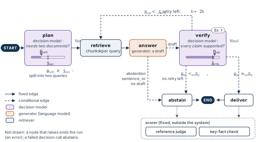
plan; the verifier’s rule (Equation 2) is the edge out of verify, which Exercise 1 writes: deliver at p_{\text{sup}} \ge \tau_{\text{verify}} = 0.8, otherwise retrieve once more with 2k chunks, otherwise abstain. The scorer sits outside the system on purpose: it grades what deliver and abstain return with its own reference judge and key-fact check, and never calls the system’s verifier. The markers on the gauges are illustrative, not measured.
The two thresholds. Both come from stated costs, following Modules 11 and 12, and both are printed in the notebook.
The planner’s two errors cost about the same. An unnecessary split costs one extra model call and a more diluted context; a missed split loses half the evidence. With equal costs, the cheaper action is the more probable one:
\text{plan}(q) = \begin{cases} \text{two queries} & p_{\text{multi}} \ge \tau_{\text{plan}} = 0.5, \\ \text{one query } (q \text{ itself}) & \text{otherwise.} \end{cases} \tag{1}
The verifier decides whether a draft reaches the participant. Treat abstention as Module 11’s deferral, at cost \ell_{\text{abs}}, and delivering an unsupported answer as a wrong action, at cost \ell_{\text{wrong}}. Chow’s rule then gives
\text{verify}(p_{\text{sup}}) = \begin{cases} \text{deliver} & p_{\text{sup}} \ge \tau_{\text{verify}} = 1 - \dfrac{\ell_{\text{abs}}}{\ell_{\text{wrong}}} = 1 - \dfrac{1}{5} = 0.8, \\[1.5ex] \text{retrieve again with } 2k \text{ chunks} & p_{\text{sup}} < \tau_{\text{verify}} \text{ and } r < R_{\max} = 1, \\[1ex] \text{abstain} & \text{otherwise.} \end{cases} \tag{2}
These are the costs of Lab 14’s stretch, and the scoring of section 3 uses the same two numbers. The rule makes two approximations, and both are worth stating. First, “supported” stands in for “correct”: a draft can be supported by a passage and still miss the question. Second, abstaining on an unanswerable question costs nothing, so abstention is cheaper on average than the rule assumes. Choosing \tau_{\text{verify}} on the development split with the capstone cost removes both approximations. That is option V1 in section 5.
Budgets. At most K_{\max} = 4 generator calls and 4 decision-model calls per question; the graph abstains when either budget is spent. Every run also sets recursion_limit, as in Lab 14.
Which model answers. The backends are chosen once, at the top of the notebook, and named on every result.
| Role | Keyed path | No key | Offline test run (CI) |
|---|---|---|---|
Generator (answer, the split in plan) |
Claude or OpenAI, by PROVIDER |
the open model (models.fallback) |
the test double, labeled stub (test double) |
Decision model (plan, verify) |
Jev, through langchain-typesafe |
the open model scored on ” yes” against ” no”, labeled Qwen log-prob decider (not Jev) |
a fixed rule, labeled stub (test double) |
| Retriever | the dense encoder of Lab 13 | the same | Lab 13’s offline stand-in, labeled stand-in (not a neural model) |
| Reference judge (the scorer’s, not the system’s) | the NLI model of Lab 13 | the same | the stub judge |
The open model is not a calibrated decision model. It is there so that the system runs without a key, and its numbers describe it, not Jev.
Check yourself. A draft comes back from the verifier with p_{\text{sup}} = 0.85 on the first attempt. (1) What does Equation 2 do? (2) A pair decides that a wrong answer should cost 10 inside their system, with abstention still at 1. What is their \tau_{\text{verify}}, and what happens to the same draft? Follow the run to its end if the second attempt gets p_{\text{sup}} = 0.88.
Answer
- 0.85 \ge 0.8: deliver. (2) \tau_{\text{verify}} = 1 - 1/10 = 0.9. Now 0.85 < 0.9 and no retry has been used (r = 0 < R_{\max} = 1), so the graph retrieves again with 2k chunks and the generator writes a second draft. That draft’s 0.88 is still below 0.9 and the retry is spent, so the system abstains, and the withheld draft stays in the record. The run used two generator calls, inside the budget of four. Whether the stricter threshold is an improvement is not decided by this trace. It will abstain on some drafts that were right. The score still charges 5 for a wrong answer, whatever the pair assumed inside the system, so the change has to be judged by \bar{\ell} on
dev.
3. The Evaluation Set and the Scoring
In this section: define the five numbers every pair reports, each with its denominator, and the single cost that combines accuracy and abstention.
The evaluation set is fixed for everyone: the same questions, scored by the same code.
- Lab 13’s question set, reused unchanged: 80 questions written and blind-checked by people, of four kinds (lookup, a fact specific to this corpus, two-part, and unanswerable).
- 45 new questions, written and checked by people under the same rules, in two kinds. Most are unanswerable, and half of those are facts a model may well know from the papers themselves but that the workshop’s pages do not state. The rest are reading-list questions that join a paper to the module and lab that use it.
- Splits:
devhas 45 questions; use it as often as you like.testhas 80; you run it twice, once for the baseline and once for your final system. About 30% of each split is unanswerable, so the abstention rate is measured on about 25 test questions rather than the 7 or 8 that Lab 13’s set alone would give.
No language model wrote, proposed, filtered or labeled any question. The reasons are Module 13’s: model-written questions copy the passage’s words, and a model that labels items is the kind of judge we are trying to check.
Five numbers. Each is reported with its denominator and Module 8’s standard error.
Accuracy on the answerable, auto-checkable questions, with an abstention counting as not correct:
\mathrm{Acc} = \frac{1}{|\mathcal{A}|} \sum_{i \in \mathcal{A}} o_i . \tag{3}
The notebook also prints the accuracy on the questions the system answered. That number rises when a system abstains more, which is why it is never reported alone.
Abstention, separately on the two kinds of question:
\mathrm{Abs}_{\mathcal{U}} = \frac{1}{|\mathcal{U}|} \sum_{i \in \mathcal{U}} \mathbf{1}[z_i = \texttt{abstain}], \qquad \mathrm{Abs}_{\mathcal{A}} = \frac{1}{|\mathcal{A}|} \sum_{i \in \mathcal{A}} \mathbf{1}[z_i = \texttt{abstain}] . \tag{4}
You want the first high (the system abstains when it should) and the second low (it does not abstain when it could have answered). Module 13 called the second the false-abstention rate.
Unsupported-answer rate: among delivered answers, the share with at least one sentence that the reference judge does not support. In Module 13’s terms, these are the answers whose faithfulness (eq. faith) is below 1:
\mathrm{Uns} = \frac{\sum_i \mathbf{1}[z_i = \texttt{answer}]\; \mathbf{1}\big[\min_j J_{\text{ref}}(a_{ij}, R_i) < \tfrac12\big]}{\sum_i \mathbf{1}[z_i = \texttt{answer}]}, \tag{5}
where a_{ij} is sentence j of the answer to question i, R_i are the passages it was written from, and J_{\text{ref}} is the reference judge: the same NLI model for every pair, fixed in the scoring code. It is deliberately not the system’s own verifier. A pair may change the verifier; nobody may change the instrument that grades it. Like every judge in Module 13, this one has not yet been compared with human labels, and the notebook says so beside its number.
Cost per question in dollars, from the token counts in every response’s usage field (Module 8, eq. cost), summed over the generator and Jev calls of the run. On the open and offline paths it is “n/a (local)”, and the number of model calls is printed instead.
Latency: the median and 95th-percentile wall-clock seconds per question.
One number for accuracy and abstention together. Accuracy and abstention pull against each other: a system that abstains on everything has a perfect \mathrm{Abs}_{\mathcal{U}} and zero accuracy. Module 13 promised to turn the pair into a cost. With the verifier’s costs,
\bar{\ell} = \frac{1}{|\mathcal{A}| + |\mathcal{U}|} \sum_{i \in \mathcal{A} \cup \mathcal{U}} \Big( \ell_{\text{wrong}}\, \mathbf{1}\big[z_i \ne \texttt{abstain}\big]\,(1 - o_i) \;+\; \ell_{\text{abs}}\, \mathbf{1}\big[z_i = \texttt{abstain}\big]\, \mathbf{1}[i \in \mathcal{A}] \Big), \qquad \ell_{\text{wrong}} = 5,\; \ell_{\text{abs}} = 1 . \tag{6}
A correct answer costs 0. A wrong answer costs 5, and so does any answer to an unanswerable question. Abstaining costs 1 on an answerable question and 0 on an unanswerable one. An error counts as a wrong answer, following Module 8’s rule; otherwise a system could abstain for free by crashing. Answerable questions without recorded key facts cannot be scored by a program, so they are left out of Equation 6 and Equation 3 and reported separately.
Worked example: the capstone cost of three systems (illustrative counts, not measurements). Take 40 auto-checkable answerable questions and 25 unanswerable ones.
| System | Cost per question \bar{\ell} |
|---|---|
| Abstain on everything: 40 abstentions at cost 1 | 40 / 65 = 0.62 |
| Answer everything, 60% correct on \mathcal{A}: 16 + 25 = 41 wrong answers at cost 5 | 205 / 65 = 3.15 |
| Answer 30 of \mathcal{A} (24 correct), abstain on the other 10; abstain on 15 of \mathcal{U} and answer 10 | (5 \times 16 + 10) / 65 = 1.38 |
With \ell_{\text{wrong}} = 5, answering pays only when the answer is right more than 1 - 1/5 = 80\% of the time: Chow’s rule again. A system that cannot tell its right answers from its wrong ones does better by abstaining. That is the role of the verifier, and the question every pair’s change has to answer.
Comparing with the baseline. Every pair’s change is measured on the same questions as the baseline, so read the difference pairwise, as in Module 13. A question is gained if its cost under Equation 6 fell and lost if it rose. If the change made no difference, each changed question would be equally likely to be a gain or a loss. The sign test asks how surprising the observed split is under that assumption:
p\text{-value} = \min\!\Big(1,\; 2 \sum_{j = \max(g, l)}^{g + l} \binom{g + l}{j}\, 2^{-(g + l)}\Big). \tag{7}
With 8 gained and 1 lost, p = 0.039. With 7 and 2 it is 0.18, and with 4 and 3 it is 1. Nine questions that change are not many, and on 80 questions a real improvement of a few points will often fail to reach 0.05. Report g, l and p together, and treat a large p as “not shown”, not as “no effect”.
The run-to-run floor. A keyed system is not deterministic: two runs of the same baseline can disagree on a few questions. Each pair therefore compares two baseline runs, its own and the instructor’s recorded one, and the notebook prints how many questions flipped between them. A change whose g + l is not clearly larger than that count has not shown anything.
Check yourself. On the worked example’s 65 questions, a fourth system answers 35 of the 40 answerable questions (26 correctly) and abstains on 5. It abstains on 20 of the 25 unanswerable questions and answers 5. (1) Compute its \bar{\ell}, \mathrm{Acc}, both abstention rates and its accuracy on the questions it answered. Is it better than the worked example’s third system? (2) Against that system it gains 6 questions and loses 1. Is the difference shown?
Answer
- Wrong answers: 9 on \mathcal{A} and 5 on \mathcal{U}, 14 in all, at cost 5; abstentions on \mathcal{A}: 5, at cost 1. So \bar{\ell} = (70 + 5)/65 = 1.15, against 1.38. \mathrm{Acc} = 26/40 = 0.65 (against 24/40 = 0.60), \mathrm{Abs}_{\mathcal{U}} = 20/25 = 0.80 (against 0.60) and \mathrm{Abs}_{\mathcal{A}} = 5/40 = 0.125 (against 0.25). Every one of the reported numbers is better. Its accuracy on answered questions is 26/35 = 0.74, lower than the third system’s 24/30 = 0.80: the one number that looks worse is the one this page says never to report alone, because it rewards abstaining. (2) By Equation 7, p = 2 \times (7 + 1)/2^7 = 0.125. Not shown at 0.05. Report g = 6, l = 1 and p = 0.125, and compare g + l = 7 with the run-to-run flip count before saying anything more.
4. The Rules of the Capstone
In this section: know what may change, what may not, and what a pair hands in.
Change one component. Choose one item from the menu in section 5, or propose your own of the same size. One change means the result can be attributed to it.
Write the hypothesis first. Before your first modified run, fill in the notebook’s hypothesis card: the component, the change, the number you expect to move, which way, and by about how much. Lab practice since Module 1 has been Predict, Run, Explain, Check; this is the Predict step for a whole system.
Develop on dev; run test twice. Run dev as often as your budget allows. Run test once for the baseline and once, at the end, for your frozen system. The notebook counts test runs and puts the count in the submission. Choosing settings on the test set makes the result optimistic: Module 11’s temperature, Module 12’s thresholds and Module 13’s chunk size were all chosen on development data for this reason.
Fixed for everyone:
- the corpus, the evaluation set, the scoring code (the notebook prints its hash) and the reference judge;
- the costs \ell_{\text{wrong}} = 5, \ell_{\text{abs}} = 1 in Equation 6 (you may use other costs inside your system, for example to set a threshold, but the score uses these);
- the models: only the IDs pinned for the workshop, with greedy decoding on the open model and the seed set in the setup cell;
- the budget: at most 4 generator calls and 4 decision calls per question, a
testrun under 10 minutes on your path, and, on a keyed path, a cost per question no more than twice the baseline’s.
Label every number. Each result carries the names of the generator, decision model, retriever and judge that produced it. Results from the offline test run are under a banner, “These numbers measure the notebook’s code, not any model”, and the instructor’s table does not rank them. A number from the open model is never reported as Jev’s.
What a pair submits is one file, written by the notebook’s last cell: the path and model names, the change and the hypothesis card, the baseline and final scores on dev and test, the gained and lost counts with the sign test, the run-to-run flip count, the cost and latency, the number of test runs, and the scoring hash. The same cell prints a share card: the five numbers before and after, and three sentences (what you changed, what you predicted, what happened). That card is your two-minute talk.
Check yourself. A pair runs test after each of five changes and submits the best of the five scores. Every one of the five runs followed the scoring rules. What is wrong with the number they report, and where will the instructor see it?
Answer
The reported score is the largest of five noisy measurements. Even if none of the five changes had any real effect, the best of five runs would often beat the baseline, because run-to-run flips and a small question set move each score a little and the pair kept the luckiest. The test set has been used to choose, which makes it a development set, and no untouched questions remain to say what the chosen system really scores. The submission file records the number of test runs, so the count of 6 (the baseline and five more) is in front of the instructor. The remedy costs nothing: iterate on dev, freeze, and run test once.
Part II. Build
11:40 to 12:25 and 13:25 to 14:30, in pairs, with lunch between. Section 5.
5. Build: One Change, Measured
In this section: improve one component of the system and measure the effect against the baseline.
A plan for the 110 minutes. Lunch falls at minute 45.
| Minutes | Do |
|---|---|
| 0–20 | Run the setup and the system self-test. Write after_verify (Equation 2, the notebook’s one exercise). Run the baseline on dev, then on test. Read ten traces: where did the system abstain, and where was it wrong? |
| 20–30 | Choose one component from the menu, using what the traces showed. Fill in the hypothesis card. |
| 30–105 | Build the change. Rerun the self-test after every edit; it must stay green. Iterate on dev. |
| 105–110 | Freeze the configuration. Do not run test yet. |
The self-test. The notebook drives the graph with a scripted generator and a scripted decision model and checks the control flow: a draft above \tau_{\text{verify}} is delivered, one below it is retried once and then abstained on, an abstention from the generator is never sent to the verifier, a split question retrieves twice, the budgets stop the run, every record names its backends, and the scoring code reproduces hand-computed numbers on hand-made records. These checks use no model, so they give the same verdict on every path. A change that breaks one has broken the system, whatever its score.
The menu. Each row gives a change, the number we expect it to move, and a guess at the size. The guesses are hypotheses, not results. Nobody has measured them on this evaluation set; finding out is the point of the capstone. Each option has a folded reference sketch in the notebook.
| Option | Component | Change | Our hypothesis (unmeasured) | Watch also |
|---|---|---|---|---|
| R1 | retrieval | hybrid retrieval: dense and BM25 fused by reciprocal rank (Lab 13’s method="hybrid") |
helps questions that hinge on a number, a symbol or a name; perhaps 0 to 3 questions gained on test |
recall@k by question kind |
| R2 | retrieval | rerank 20 candidates with the cross-encoder or Jev (Lab 13, Exercise 4) | the first useful passage moves up; perhaps 0 to 4 questions gained | latency; with Jev, about 20 more decision calls per question |
| R3 | retrieval | change k or the chunk size from Lab 13’s choice | more passages raise recall but can lower accuracy and raise cost in proportion | cost per question |
| P1 | prompt | stricter abstention instruction, or “quote the supporting sentence, then answer” | \mathrm{Abs}_{\mathcal{U}} up by 10 to 30 points, and \mathrm{Abs}_{\mathcal{A}} up too; the sign of the change in \bar{\ell} is the open question | false abstentions |
| P2 | prompt | one worked example of a cited answer and one of an abstention | as P1, with fewer uncited sentences | prompt length and cost |
| V1 | threshold | choose \tau_{\text{verify}} on dev by minimizing Equation 6 (Module 11, eq. selective-cost) |
lowers \bar{\ell} a little if the verifier is informative. If it is not (likely for the 0.5B open model), the best threshold runs to 0 or 1, and that is a finding about the verifier | the verifier’s reliability diagram on dev |
| V2 | control | three regions for the verifier: deliver, retry, or abstain at once (Lab 12’s action_thresholds, with retrying as the “ask” action) |
saves calls on hopeless drafts at little cost in accuracy | calls per question |
| V3 | control | retry policy: R_{\max} = 0 or 2, or retry with a rewritten query instead of 2k | retries recover a few answerable questions and cost 30 to 50% more | cost, latency |
| G1 | routing | tune \tau_{\text{plan}} or the splitting prompt | affects only the two-part and reading-list questions, about 20 on test; the effect will probably be below the noise, which is itself worth reporting |
split rate by question kind |
| T1 | tool | replace the fixed retrieve step with Lab 14’s tool-calling agent node and a search_docs tool, so the model writes its own queries |
helps two-part questions, at 2 to 3 times the calls; watch for loops | calls per question against K_{\max} |
| M1 | generator | the other pinned provider, if you have both keys | probably the largest change of any option, in accuracy and in cost; the verifier threshold was set for the first generator | cost per question |
Two changes are not allowed in the scored run: adding documents to the corpus, which would turn unanswerable questions into answerable ones, and changing the reference judge or the scoring code.
Optional: For Instructors, How to Circulate During the Build
- At minute 20, check that every pair has a baseline on
devand has read traces. A pair choosing a component without having looked at failures is guessing. - Steer toward the failures. If the two-by-two table of Module 13 shows mostly retrieval failures, a prompt change is unlikely to help, and the reverse is also true.
- Watch the budget on keyed paths. A reranker with Jev, or a tool-calling node, multiplies calls. A room of pairs on one shared key can hit rate limits that we have not been able to measure.
- Encourage null results. A well-measured “no difference” with g, l and p is a good share. A large claimed gain with g + l below the flip count is not.
Part IV. Wrap-Up
16:30 to 17:00, the whole room, ending in the day’s closing slot. Sections 7 to 10.
7. Five Days, One Line of Ideas
In this section: say, for each module, which limitation of the previous one it removed.
Each module began where the last one stopped working. Where a lab measured the step on the running thread, the number is in the table: test-split results from data/baselines.json, run on CPU in the build environment.
| Module | What it added | Measured on the running thread | What it left open, and who took it up |
|---|---|---|---|
| 1 · Text as data | counts: n-gram language models, TF-IDF and a linear classifier | character 5-gram perplexity 6.25; topic accuracy 0.884 | words are unrelated symbols, and the context is a fixed window → 2 |
| 2 · Word vectors | dense vectors learned from context; the first neural language model | averaged embeddings 0.867: no better than TF-IDF on this task | averaging discards order; the window is still fixed → 3 |
| 3 · Sequence models | a state carried over any length; gating against vanishing gradients | LSTM perplexity 5.01 | a whole input squeezed into one vector, read one step at a time → 4 |
| 4 · Seq2seq and attention | the decoder looks back at every encoder state | recurrence is still sequential, and attention runs only from decoder to encoder → 5 | |
| 5 · The transformer | self-attention everywhere, in parallel | mini-GPT perplexity 4.70, against 4.82 for the LSTM trained under the same budget | tiny, character-level, trained from scratch on 1 MB → 6 |
| 6 · Pretraining | subword tokens; pretrain once on unlabeled text, reuse many times | a pretrained model continues text; it does not follow instructions → 7 | |
| 7 · Fine-tuning and LoRA | instruction tuning, cheaply, with low-rank updates | the largest models are reached only through APIs, with structured output and tools → 8 | |
| 8 · LLMs through APIs | structured output, a tool loop, one evaluation harness | no label for “better”, and a fluent answer carries no confidence signal → 9 | |
| 9 · Preference learning | the policy gradient; a reward model learned from comparisons | a policy optimized against a learned reward exploits it → 10 | |
| 10 · RLHF | KL-regularized optimization; DPO without a reward model | it optimizes what raters prefer, and raters do not judge confidence → 11 | |
| 11 · Calibration | what a probability should mean; temperature scaling; abstention by cost | ECE 0.164 → 0.009 after temperature scaling (the C = 1 classifier) | the fix comes after training, and there are only two actions → 12 |
| 12 · RLCD and Jev | calibration as a training target (RLCD: TypeSafe’s stated name and aim; the method is unpublished, and Lab 12’s toy is our illustration); typed decisions with probabilities; act, ask, escalate | a decision is only as good as the state in front of it → 13 | |
| 13 · RAG | retrieval puts the right documents in the state; retrieval and answers measured separately | a fixed pipeline: no branching, no actions, no pause for a person → 14 | |
| 14 · Agents | an explicit graph with state, interrupts, a router and a guard | parts measured one at a time; the whole never measured on a fixed task → 15 | |
| 15 · Capstone | one system, measured end to end for accuracy, abstention and cost | your table | section 9 |
Three threads run through the table.
- Every step was motivated by a measured failure, and the running thread is what made the measurement possible. Some steps did not win on every metric: averaged embeddings lost to TF-IDF on topic classification. Measuring is how we know.
- Days 1 and 2 asked what a model predicts; Days 3 to 5 asked when to trust it. Preference learning shaped what models say, calibration asked whether their probabilities mean anything, and the capstone used those probabilities to decide whether to speak at all.
- The unit of evaluation grew. It went from a perplexity on one corpus, to a classifier’s accuracy, to a reliability diagram, to a system’s cost per question. At each step the evaluation had to be designed before the model.
8. An Evaluation Checklist for Agentic Systems
In this section: apply a checklist that makes an agentic system’s evaluation trustworthy.
Each item names the module where you met it.
- Write the task contract first: what counts as correct, and when the system must abstain (15).
- Use a fixed evaluation set, written and checked by people, with answerable and unanswerable items and no model-written items or labels (11, 13, 15).
- Choose on development data and report on test data, once per configuration (11, 12, 13).
- Measure the parts, then the whole. Measure retrieval recall, router accuracy and verifier calibration, and then end-to-end accuracy and abstention. Reliability compounds: if each of ten steps succeeded independently 95% of the time, the run would succeed 0.95^{10} \approx 60\% of the time. Real steps are not independent, which is why the whole must be measured directly (13, 14, 15).
- Report the denominator and the standard error. Compare pairwise, with gained and lost counts and a sign test, and know the run-to-run variation of a stochastic system (8, 13, 15).
- Count invalid outputs and errors as wrong (8, 15).
- Report cost and latency per task beside quality, measured from the providers’ usage counts, not estimated (8, 15).
- Set thresholds from stated costs and print them. Compare them with probabilities, not with a “confidence” field (11, 12, 14).
- Check the calibration of every probability you act on, in its role and on its own domain (11, 12, 14).
- Treat judges as models. Pin them, keep them separate from the system’s own checks, and validate them against human labels (8, 13, 15).
- Test attacks, not only answers. Measure direct and indirect prompt injection, and the unsafe-action rate, both attempted and carried out (8, 14).
- Count the human’s work. Every interrupt costs a person’s time, and a simulated human who never misses anything is optimistic (12, 14).
- Label every number with the system that produced it. A stand-in’s number must never travel as a result (8, 11–15).
- Version everything that can change a number: model IDs, package pins, prompts, the corpus and the evaluation set. Re-run when any of them changes (all).
Check yourself. Item 4 says that ten steps which each succeed 95% of the time, independently, give a run that succeeds about 60% of the time. Under the same assumption, how reliable must each of ten steps be for the run to succeed 90% of the time? What does the answer say about where to spend effort in a long pipeline?
Answer
Each step must succeed with probability 0.9^{1/10} = 0.9895, about 99%: the failure rate per step has to fall from 5% to about 1%, a factor of five, to move the run from 60% to 90%. Check: 0.99^{10} = 0.904. Two things follow. Shortening the pipeline helps as much as improving a step, since each step removed takes one factor out of the product. And a step that can detect its own likely failures and abstain, ask or escalate, as the verifier and the guard do, turns a silent error into a visible and cheaper one, which the product of success rates does not show. Real steps are not independent, so treat the arithmetic as a warning and measure the whole run.
9. Open Problems
In this section: name questions the workshop raised and could not close.
- Calibration under shift. Module 14’s bound on unsafe actions holds only on the distribution the guard was calibrated on. Making probabilities stay meaningful on new domains, and under attack, is open. Kamath et al. (2020) show the problem for question answering.
- Prompt injection. There is no complete defense inside the model. Today’s defenses are architectural, and they limit what injected text can cause rather than preventing it (Module 14).
- Judges. Faithfulness and answer quality are scored by models whose agreement with people is often unmeasured. Building cheap, validated judges is unsolved, and a supported answer can still be wrong.
- Reward models and raters. Reward hacking and sycophancy (Module 10) persist when a model is optimized against any learned proxy for what people want.
- Training for calibrated decisions. TypeSafe states that its System One models “are trained for calibrated decisions” and has not published how. Whether such training transfers across domains is a question anyone can test with a key and a labeled set, and TypeSafe’s own advice is to “validate their performance in the target domain”. Our Lab 12 toy shows what a proper-score reward does on a small model; it says nothing about Jev.
- Evaluating agents. Benchmarks that report only accuracy reward needlessly costly systems. Kapoor et al. (2024) argue for reporting cost beside accuracy and for held-out tests. Agent evaluations are also expensive to repeat, which makes the run-to-run variation hard to pin down.
10. Further Study
- Courses. The three this workshop calibrated against: Stanford CS224N, CMU CS 11-747 and MIT 6.S191 (see References).
- A textbook. Jurafsky and Martin, Speech and Language Processing, 3rd edition draft, especially the chapters on question answering and information retrieval.
- Building agent systems. Andrew Ng’s course Agentic AI (DeepLearning.AI, 2025) teaches reflection, tool use, planning and multi-agent patterns in plain Python, with a module on evals and error analysis. Anthropic’s Claude Certified Architect – Foundations exam guide (2026) is a compact syllabus for production agent design: loops and stopping, coordinators and subagents, tool design and MCP, enforcement and hand-offs, context and escalation. Its free preparation courses are public; the certification itself is currently open only to organizations in the Claude Partner Network. The guide names Anthropic’s tools throughout; its design questions apply with any provider. See References, Module 14.
- Evaluation. The readings below, starting with Liang et al. (2023) and Dror et al. (2018).
- The systems you used. Re-read the current documentation of the providers, LangGraph, LlamaIndex and TypeSafe before you build on them. Every page of this workshop that names a version gives the date it was checked.
- Your own corpus. Point the capstone at documents you know, write 50 questions yourselves, including unanswerable ones, and run the checklist of section 8.
Equations and Where You Implement Them
| Equation | Lab 15 |
|---|---|
| Planner rule (Equation 1) | provided: after_plan, with \tau_{\text{plan}} printed; changed in option G1 |
| Verifier rule (Equation 2) | the exercise: after_verify, checked by the self-test with a scripted decision model; \tau_{\text{verify}} printed; changed in options V1 and V2 |
| Accuracy (Equation 3), abstention (Equation 4), unsupported answers (Equation 5), capstone cost (Equation 6) | provided, fixed for everyone: score(records) in the scoring cell, whose hash appears in every submission; the self-test checks it against hand-computed values |
| Sign test (Equation 7) | provided: compare(baseline, final), with g, l, p and the run-to-run flip count on the share card |
Summary
- The capstone is a research assistant over the workshop’s own pages, with a contract: a cited answer, or the exact abstention sentence. Answering from memory breaks the contract.
- The starter system is a plan–retrieve–answer–verify graph built from Labs 12 to 14. A decision model plans and verifies, and both thresholds come from stated costs (Equation 1, Equation 2).
- The evaluation set is fixed and written by people: Lab 13’s 80 questions plus 45 new ones, about 30% unanswerable, with a
devsplit for development and atestsplit run twice. - Report accuracy, abstention on both kinds of question, the unsupported-answer rate, cost and latency, each with its denominator (Equation 3, Equation 4, Equation 5). The capstone cost combines accuracy and abstention into one number (Equation 6).
- Compare with the baseline pairwise, with the sign test (Equation 7), against the run-to-run variation of the baseline itself.
- Change one component, predict first, develop on
dev, and report what happened, including nothing. - The five days form one line: each module removed a limitation of the last, and the evaluation grew from a perplexity to a system’s cost per question.
Gotchas and Troubleshooting
- “Abstaining is a failure.” On an unanswerable question it is the right answer. The capstone cost charges abstention only where an answer existed, and charges a wrong answer five times as much.
- “Accuracy on answered questions is the headline number.” It rises when a system abstains more. Report it beside accuracy on all answerable questions and both abstention rates.
- “The verifier and the scorer can be the same model.” Then a pair could raise its score by loosening its own verifier. The scorer’s judge is fixed, separate and the same for everyone.
- “A correct answer from the model’s memory is fine.” Not under this contract. It cannot be checked against a source, and the user cannot tell it from an invented one.
- “Seven gained and two lost is a clear win.” The sign test gives p = 0.18. Read gained and lost counts with their test, and against the run-to-run flips of the baseline.
- “Running
testafter every change is just more data.” It turns the test set into a development set and makes the final number optimistic. - “The Qwen decider’s results tell us about Jev.” They describe a 0.5B open model scored on yes and no. Only the keyed path measures Jev, and only on these questions.
- “A bigger change always wins.” Swapping the generator may move accuracy most, at a cost the score does not include. Report dollars and seconds beside the score.
Next Steps
There is no Module 16. The checklist of section 8 and the starter system are yours to take to your own documents. When you do, write your own questions, unanswerable ones included, before you build anything.
Further Reading
- Kapoor, S., Stroebl, B., Siegel, Z. S., Nadgir, N. and Narayanan, A. (2024). AI Agents That Matter. arXiv:2407.01502 (reported as published in TMLR, 2025). Why agent evaluations must report cost beside accuracy, use held-out tests and be reproducible. Title, authors and summary checked by web search on 2026-10-05; the TMLR venue was seen only in a search summary.
- Rajpurkar, P., Jia, R. and Liang, P. (2018). Know What You Don’t Know: Unanswerable Questions for SQuAD. ACL (short papers). The case for putting unanswerable questions in an evaluation set, and how far a system that cannot abstain falls. Checked by web search.
- Kamath, A., Jia, R. and Liang, P. (2020). Selective Question Answering under Domain Shift. ACL. Abstention in question answering, why a model’s own probabilities are a poor abstention signal off its domain, and a separate calibrator that does better. Checked by web search.
- Dror, R., Baumer, G., Shlomov, S. and Reichart, R. (2018). The Hitchhiker’s Guide to Testing Statistical Significance in Natural Language Processing. ACL. Which test to use when two systems are compared on the same examples. Checked by web search.
- Liang, P., Bommasani, R., Lee, T., Tsipras, D. et al. (2023). Holistic Evaluation of Language Models. TMLR. Evaluating models on several metrics at once (accuracy, calibration, robustness, efficiency and more) rather than one. Checked by web search.
Also used above: Modules 8 and 11 to 14 of this workshop; typesafe-ai/skills, SKILL.md (the TypeSafe statements quoted in sections 7 and 9, read for briefs/jev-verification.md).