viewof obj06 = Inputs.radio(["masked (BERT)", "causal (GPT)"], {label: "Objective", value: "masked (BERT)"})
viewof rate06 = Inputs.range([0.05, 0.6], {label: "Selection rate (masked)", step: 0.05, value: 0.15})
viewof draw06 = Inputs.range([1, 30], {label: "Random draw (masked)", step: 1, value: 1})
viewof pos06 = Inputs.range([2, 12], {label: "Predicted position t (causal)", step: 1, value: 6})Pretraining and the Hugging Face Stack
Subword tokenization, masked and causal pretraining, and using pretrained models through Hugging Face.
Open the lab in Colab Hugging Face PyTorch
- Duration
- 120 minutes (55 briefing, 55 lab, 10 debrief)
- Level
- 300 · Advanced
- Lab runtime
- Google Colab, free T4 GPU · about 7 minutes of compute
- Accounts and cost
- Google. Free
- Without API keys
- an open model runs in place of the commercial one
What You Will Build
In this module you will:
- Explain subword tokenization and the masked and causal pretraining objectives
- Load, inspect and run pretrained models with Hugging Face
- Configure a supplied fine-tuning run for an encoder classifier and evaluate it against Labs 1 and 2
New terms, in the glossary: pretraining, fine-tuning, model checkpoint.
Before You Start
- Module 5 · The Transformer and its lab, and the modules before it: this module measures its results against theirs.
- A Google account, and the Colab runtime set to T4 GPU (Runtime → Change runtime type).
- API keys are optional. Without them an open model runs in place of the commercial one.
Where we are. Module 5 built a decoder-only transformer and trained it from random parameters on one megabyte of text, one character at a time. The architecture was sound; the data and the token were the limits. This module answers one question: how do we train a transformer once, on far more text and with a better token, so that every later task starts from what it learned?
In the Lab
5 exercises in 3 parts. The notebook budgets 47 minutes for them; the lab slot is 55 minutes. Each exercise you write is a # TODO stub with a folded solution beneath it and a checkpoint that passes or fails; where people tend to stall, a folded hint sits above the stub.
| Task | Briefing section | Time |
|---|---|---|
| Part A · Subword Tokenization | ||
| Exercise 1 · Byte-Pair Encoding by Hand | 2 | 10 min |
| Exercise 2 · Train a Tokenizer and Count Tokens per Word | 2, 6 | 7 min |
| Part B · Two Pretraining Objectives | ||
| Exercise 3 · Causal Language Modeling and Perplexity | 4 | 8 min |
| Exercise 4 · Masked Language Modeling: Select and Corrupt | 5 | 10 min |
| Part C · Fine-Tuning for Classification | ||
| Exercise 5 · Fine-Tune an Encoder | 7 | 12 min |
Challenge · Attention and Hidden States of a Pretrained Encoder
Optional, for anyone who finishes the core path early: the notebook’s stretch section, after the last checkpoint.
When you are done. Runtime → Disconnect and delete runtime releases the machine; your keys stay in Colab Secrets for the next lab.
Agenda
| Minutes | Section | In the room |
|---|---|---|
| 0–3 | 1. What the From-Scratch Transformer Leaves Open | — |
| 3–16 | 2. Subword Tokenization: Byte-Pair Encoding | Check yourself (2 min) |
| 16–19 | 3. Pretrain Once, Reuse Many Times | — |
| 19–27 | 4. Causal Language Modeling: GPT | Check yourself (2 min) |
| 27–38 | 5. Masked Language Modeling: BERT | Demo (4 min) |
| 38–43 | 6. The Hugging Face Stack | — |
| 43–55 | 7. Fine-Tuning an Encoder for Classification | Check yourself (2 min) |
| 55 | Total | 45 minutes of exposition, 10 of activities |
Checks, demos and predictions listed here are part of the live session and its minutes; the others on the page are for reading afterwards.
Read now · Sections 1–7, in the agenda above.
Use in the lab · Exercise 1: section 2; Exercise 2: sections 2 and 6; Exercise 3: section 4; Exercise 4: section 5; Exercise 5: section 7.
Read later · Section 8, What Changes at Scale, and What Is Still Missing (Reference); the collapsed callouts marked Optional; Further Reading.
The lab exercise each section prepares is listed in the equation-to-lab map at the end of the page.
Notation for This Module
Notation carried over from earlier modules: tokens w_1, \dots, w_T; vocabulary V of size |V|; embedding e_w \in \mathbb{R}^d; logits z and \hat{y} = \mathrm{softmax}(z); parameters \theta; loss \mathcal{L}; perplexity \mathrm{PPL}; number of classes C. All logarithms are natural. New in this module:
| Symbol | Meaning |
|---|---|
| M | number of merges learned by byte-pair encoding (not Module 5’s causal mask, which this page names only in words) |
_ |
end-of-word symbol used in the BPE examples |
| h_t \in \mathbb{R}^d | the transformer’s output vector at position t (its last layer), a contextual embedding |
| \theta_{\text{pre}} | parameters after pretraining |
| \mathcal{L}_{\text{CLM}}, \mathcal{L}_{\text{MLM}} | causal and masked language-modeling losses |
| \mathcal{S} | the set of positions selected for prediction in masked language modeling |
| \tilde{w}_1, \dots, \tilde{w}_T | the corrupted input sequence in masked language modeling |
[CLS], [SEP], [MASK], [PAD] |
BERT’s special tokens: sequence start, separator, mask, padding |
| h_{\texttt{[CLS]}} | the output vector at the [CLS] position |
| \eta | learning rate |
1. What the From-Scratch Transformer Leaves Open
Objective: name the two limits of Lab 5’s model that this module removes.
In Module 5 you trained a decoder-only transformer on one megabyte of Shakespeare and compared it with Lab 3’s LSTM on the same test split. Whatever the margin, it is still a weak model of language, for two reasons that have nothing to do with the architecture.
The data is tiny. One million characters is about 182,000 words (181,780 whitespace-separated words in the training split, measured). Everything the model knows about English, it learned from that. It has never seen the word gradient. Starting from random parameters, every new task would have to relearn the language from its own small dataset.
The token is the wrong size. Module 1 offered two units and both are poor:
| Unit | Vocabulary | Sequence length | Unknown tokens |
|---|---|---|---|
| Characters | tiny (65 in Lab 5) | long: 5.5 tokens per word on Tiny Shakespeare and 7.3 on the arXiv abstracts, counting the space (measured) | none |
| Words | large, and never complete (Zipf’s tail) | short | every new word becomes <unk> |
Length matters more for a transformer than for an RNN, because self-attention compares every position with every other: cost grows as T^2. A character model also spends capacity learning to spell before it can learn anything else. A word model cannot represent pretraining if it only saw train.
This module answers both. Section 2 builds a token between the character and the word. Sections 3 to 5 train the same transformer on billions of words once, with a loss that needs no labels, and reuse the result. Sections 6 and 7 do that reuse in practice, on the classification task you have carried since Lab 1.
2. Subword Tokenization: Byte-Pair Encoding
Objective: state the BPE algorithm precisely enough to implement it, and say what its one hyperparameter trades.
The idea. Keep frequent words whole and split rare words into frequent pieces. Then the vocabulary has a fixed size that we choose, common words cost one token, and a word never seen before is still representable as a sequence of pieces. The pieces are called subwords.
Byte-pair encoding (BPE) learns the pieces from data. Gage (1994) proposed it for data compression; Sennrich et al. (2016) applied it to words. Start from characters and repeatedly glue together the most frequent adjacent pair.
Learning the Merges
Input: a training corpus and the number of merges M.
- Pre-tokenize. Split the corpus into words (on whitespace, say) and count them. The algorithm runs on this table of word counts, so pairs never cross a word boundary.
- Initialize. Write each word as a sequence of single characters followed by an end-of-word symbol, which we write
_. The initial vocabulary V_0 is the set of all symbols that appear. - Repeat M times:
- Count pairs. For every pair of adjacent symbols (a, b), add up the counts of the words it occurs in, once per occurrence.
- Pick the pair with the highest count. Break ties by a fixed rule; ours is the pair that sorts first.
- Merge. In every word, replace each occurrence of a followed by b with the single new symbol ab, scanning left to right.
- Record. Add ab to the vocabulary and append (a, b) to the merge list.
Output: the ordered merge list. The final vocabulary has
|V| = |V_0| + M \tag{1}
symbols, because each merge adds exactly one. M is the only hyperparameter.
As code, with the two functions you write in the lab left out:
def train_bpe(word_freqs, num_merges):
    # word_freqs: {"low": 5, ...}  ->  {("l", "o", "w", "_"): 5, ...}
    words = {tuple(w) + ("_",): f for w, f in word_freqs.items()}
    merges = []
    for step in range(num_merges):
        counts = pair_counts(words)                         # step 3a
        if not counts:
            break                                           # every word is one symbol
        best = min(counts, key=lambda p: (-counts[p], p))   # step 3b, ties sort first
        words = merge_pair(words, best)                     # step 3c
        merges.append(best)                                 # step 3d
    return merges
A Worked Example
A corpus of four words with their counts (the example of Sennrich et al.): low 5, lower 2, newest 6, widest 3. The initial vocabulary has 11 symbols: d e i l n o r s t w _.
| Merge | Pair chosen | Count | The words afterwards |
|---|---|---|---|
| start | l o w _ · l o w e r _ · n e w e s t _ · w i d e s t _ |
||
| 1 | e + s |
9 | l o w _ · l o w e r _ · n e w es t _ · w i d es t _ |
| 2 | es + t |
9 | l o w _ · l o w e r _ · n e w est _ · w i d est _ |
| 3 | est + _ |
9 | l o w _ · l o w e r _ · n e w est_ · w i d est_ |
| 4 | l + o |
7 | lo w _ · lo w e r _ · n e w est_ · w i d est_ |
| 5 | lo + w |
7 | low _ · low e r _ · n e w est_ · w i d est_ |
Check merge 1: the pair e s occurs in newest (6) and widest (3), so its count is 6 + 3 = 9. The pairs s t and t _ also have count 9; the tie rule picks e s. After five merges the vocabulary has 11 + 5 = 16 symbols (Equation 1), and the algorithm has found a suffix, est_, and a stem, low, without being told what either is.
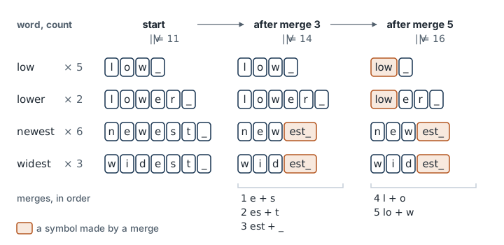
est_ is one symbol; after five, so is the stem low. Each merge adds one symbol to the vocabulary, so |V| goes from 11 to 14 to 16 (Equation 1).
Encoding a New Word
To tokenize a word, split it into characters plus _, then apply the merges in the order they were learned.
lowest was not in the corpus:
l o w e s t _ → (1) l o w es t _ → (2) l o w est _ → (3) l o w est_ → (4) lo w est_ → (5) low est_
Two known pieces, low and est_, and no unknown token. A word made only of rare pieces falls back toward characters: with these five merges, newer stays n e w e r _. That is the pricing rule: frequent words cost one token, rare words cost several.
What the Hyperparameter Trades
- M = 0 is a character model. M \to \infty merges every training word into one symbol: a word model.
- In between, larger M gives shorter sequences and a larger embedding table and output layer, each with |V| rows.
- Real models sit between these extremes. GPT (2018) used 40,000 merges. GPT-2 uses a vocabulary of 50,257. BERT’s vocabulary has about 30,000 entries.
Real Tokenizers
Real tokenizers run this algorithm with three differences of detail: where the word boundary is marked (GPT-2’s Ġ marks the start of a word, BERT’s ## marks a piece that continues one), what the base symbols are (GPT-2’s byte-level BPE starts from the 256 byte values, so no string is unknown), and how the pair to merge is chosen (BERT uses WordPiece). The pieces they find are frequent strings, not morphemes. The optional box below gives the details and the same sentence under two pretrained tokenizers; Exercise 2 prints the real splits.
Optional: Three Things That Differ Between Real Tokenizers
- Where the word boundary is marked. We put
_at the end of a word. GPT-2 marks the start of a word by attaching the preceding space to it (shown asĠwhen you print tokens). BERT marks pieces that continue a word with a##prefix. - What the base symbols are. GPT-2 uses byte-level BPE: the base vocabulary is the 256 possible byte values, so any string in any script can be encoded and there is no unknown token. Its 50,257 entries are 256 bytes, 50,000 merges and one end-of-text token.
- How merges are chosen. BERT uses WordPiece, which picks pairs by a different criterion (the optional WordPiece box after the check-yourself questions). The result looks similar.
The same sentence under two pretrained tokenizers. These splits illustrate each tokenizer’s conventions; they have not been reproduced in the workshop build, because the build machine cannot reach the Hugging Face Hub. Exercise 2 prints the real ones, and they may differ in detail.
We fine-tune a pretrained transformer for multilingual summarization.

BERT (WordPiece, lowercased):
  we fine - tune a pre ##train ##ed transform ##er for multi ##ling ##ual sum ##mar ##ization .
GPT-2 (byte-level BPE):
  We Ġfine - t une Ġa Ġpret rained Ġtransformer Ġfor Ġmult ilingual Ġsummar ization .
Expect splits that do not follow the morphology a linguist would draw (in the illustration, Ġpret + rained); check this against the real output in Exercise 2. The pieces are frequent strings, not meanings. The model learns what to do with them.
A tokenizer belongs to its model. The embedding matrix has one row per token ID. A model pretrained with one tokenizer and fed IDs from another receives the wrong rows, and nothing raises an error. Always load the tokenizer from the same checkpoint as the model.
Tokens are not words. From here on, T counts subword tokens. On the workshop’s arXiv Topics set the median training text has 183 words (measured). The BPE tokenizer you train in Exercise 2, with |V| = 4{,}000 on the 4,800 training texts, needs 1.548 tokens per word on the validation texts (measured), so at that rate a median text is roughly 280 tokens. Exercise 2 measures the same ratio for the two pretrained tokenizers; those values have not yet been measured for this page. Context limits, cost and truncation are all counted in tokens.
In the lab. In Exercise 1 you write pair_counts(words) (step 3a) and merge_pair(words, pair) (step 3c); the checkpoint is the table above (first merges e+s, es+t, est+_, l+o, lo+w), the encoding of lowest and |V| = 11 + 5. In Exercise 2 you write tokens_per_word(encode_fn, texts), train a BPE tokenizer on the arXiv training texts with the tokenizers library, and compare it with the two pretrained tokenizers above by tokens per word on the validation texts.
Check yourself. Continue the worked example by one step. After merge 5 the words are low _ (5), low e r _ (2), n e w est_ (6) and w i d est_ (3). Which pair does merge 6 choose, with what count, and what decided it?
Answer
e + w, with count 6. Three pairs tie at 6, all of them inside newest: (e, w), (n, e) and (w, est_). Every pair that involves low now counts less (low + _ is 5, low + e is 2). The tie rule picks the pair that sorts first, (e, w), so newest becomes n ew est_ and the vocabulary has 11 + 6 = 17 symbols. A different tie rule would give a different vocabulary from the same data, so the rule is part of the tokenizer.
Check yourself. Neither slowest nor lowers is in the toy corpus. Encode both with the five merges of the table. Which costs more tokens, and why?
Answer
slowest becomes s low est_: 3 tokens. lowers becomes low e r s _: 5 tokens. The longer word is cheaper because it is made of two pieces the corpus made frequent, plus one leftover character. In lowers, only low is a learned piece: no merge ever joined e r, r s or s _, so the rest falls back to characters. Cost follows the frequency of the pieces in the training corpus, not the length of the word.
Optional: WordPiece
WordPiece (used by BERT and DistilBERT) also builds a vocabulary by merging pairs, bottom up. It differs from BPE in two places.
Choosing the pair. Instead of the raw pair count, WordPiece scores a pair by its count relative to the counts of its parts:
\mathrm{score}(a, b) = \frac{c(a, b)}{c(a)\, c(b)},
where c(a, b) is the count of the adjacent pair and c(a), c(b) the counts of the two symbols. A pair scores high when its parts occur together more often than their individual frequencies would suggest. BPE merges the pair that is most frequent; WordPiece merges the pair that is most associated. Google did not release its WordPiece training code; this description is the reconstruction given in the Hugging Face documentation and course (Readings, item 5).
Encoding a word. WordPiece does not replay merges. It stores only the final vocabulary and tokenizes greedily: take the longest prefix of the word that is in the vocabulary, then the longest piece that continues from there, and so on. Pieces after the first carry the ## prefix. If some part of the word cannot be matched, the whole word becomes [UNK], so, unlike byte-level BPE, WordPiece can produce unknown tokens.
A third family, Unigram (used by T5 through the SentencePiece library), starts from a large candidate vocabulary and prunes it. All three produce subword vocabularies of a chosen size; the differences rarely matter to a user of a pretrained model.
3. Pretrain Once, Reuse Many Times
Objective: state the transfer-learning recipe and say which part of it you have already seen.
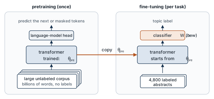
In Lab 2’s stretch section, pretrained GloVe vectors replaced the embeddings you trained yourself. That was transfer of one layer: the embedding matrix E. Each word still had a single vector regardless of its sentence, and everything above E started from random.
A transformer turns the embeddings e_{w_1}, \dots, e_{w_T} into output vectors h_1, \dots, h_T, where each h_t \in \mathbb{R}^d depends on the whole input through self-attention. These are contextual embeddings: bank gets a different h_t in river bank and bank loan. The proposal is to transfer the whole network that computes them.
The recipe has two stages.
- Pretraining. Train the transformer on a very large corpus of plain text with a self-supervised objective: one whose targets are made from the text itself, so no human labels are needed. The result is a set of parameters \theta_{\text{pre}}. This is done once, at great cost, usually by someone else.
- Fine-tuning. Copy \theta_{\text{pre}}, add a small task-specific output layer, and continue training on the labeled data of the task. This is cheap: minutes on one GPU.
What should the self-supervised objective be? Two answers dominate, and they correspond to the two halves of the original transformer. Recall from Module 5 that a block with a causal mask lets position t attend only to positions \le t, and a block without the mask lets every position attend to every other.
| Causal language modeling | Masked language modeling | |
|---|---|---|
| Architecture | decoder-only (causal mask) | encoder-only (no mask) |
| Each position sees | the left context | both sides |
| Example | GPT (Radford et al., 2018) | BERT (Devlin et al., 2019) |
| Natural use | generating text | classifying and tagging text |
Check yourself. Lab 2 trained skip-gram embeddings by predicting the words around a center word. Is that objective self-supervised, by this section’s definition? If so, what is new in the recipe above?
Answer
Yes. The targets, the context words, are made from the text itself, and no person labeled anything. What is new is how much is transferred. Skip-gram hands on one table with one vector per word, the same in every sentence. Pretraining hands on the whole network that computes the contextual vectors h_t, so fine-tuning starts with every layer already trained and only the small task layer random.
4. Causal Language Modeling: GPT
Objective: write the causal objective and recognize it as Module 1’s.
You already know this objective. Module 1 factorized the probability of a text with the chain rule, with no approximation:
P(w_1, \dots, w_T) = \prod_{t=1}^{T} P(w_t \mid w_{<t}).
A causal language model (CLM) computes each factor with a decoder-only transformer. The output vector at position t - 1 passes through the output layer of Modules 3 and 5 to give logits over the vocabulary, z_{t-1} = W_o h_{t-1} + b_o, and P_\theta(w_t \mid w_{<t}) is entry w_t of \mathrm{softmax}(z_{t-1}). The loss is the average negative log-probability of each token given the tokens before it:
\mathcal{L}_{\text{CLM}}(\theta) = -\frac{1}{T} \sum_{t=1}^{T} \log P_\theta(w_t \mid w_{<t}), \qquad \mathrm{PPL} = \exp\bigl(\mathcal{L}_{\text{CLM}}\bigr). \tag{2}
This is the cross-entropy you minimized in Lab 5, and its exponential is the perplexity of Module 1. (The first token has no left context unless a start token is placed before it. The library’s loss, and the lab, average over positions 2 to T.) GPT is the mini-GPT of Lab 5 with three changes, none of them to the equations:
| Lab 5 mini-GPT | GPT (2018) | |
|---|---|---|
| Tokens | 65 characters | BPE, 40,000 merges |
| Data | 1 MB of Shakespeare | BooksCorpus, over 7,000 books |
| Model | a few layers | 12 layers, 768 dimensions, 12 heads |
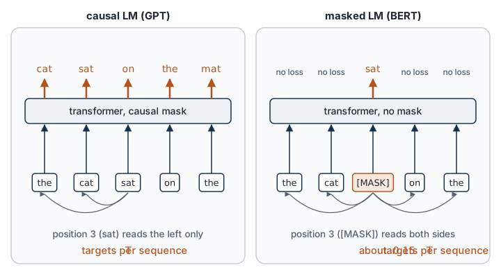
Why it is efficient. With the causal mask, one forward pass yields a prediction at every position, and every position has a target (the next token). A sequence of T tokens gives T training signals.
What it gives up. h_t summarizes only w_1, \dots, w_t. For generation that is exactly right. For understanding a whole sentence it is a handicap: the representation of bank in bank of the river is computed before the model has read river.
Perplexity across tokenizers. Module 1 warned that perplexities are comparable only over the same tokens. GPT-2’s perplexity is per BPE token and Lab 5’s is per character, so the two numbers cannot be compared directly. The total negative log-probability of a text, T \cdot \mathcal{L}_{\text{CLM}}, does not depend on the unit. Divide it by the number of characters to get nats per character under either model.
Worked example: one text, two units. A text of 12 characters is 3 BPE tokens. A causal LM gives the three tokens probabilities 0.5, 0.25 and 0.125, each conditioned on the tokens before it. (Assume a start token, so that all three are scored.)
- Loss (Equation 2): \mathcal{L}_{\text{CLM}} = \tfrac{1}{3}(\log 2 + \log 4 + \log 8) = 2 \log 2 \approx 1.386 nats per token.
- Perplexity: \exp(2 \log 2) = 4. On average the model is as uncertain as a uniform choice among 4 tokens.
- Total: 3 \times 1.386 = 4.159 nats for the whole text. This number does not depend on the unit.
- Per character: 4.159 / 12 \approx 0.347 nats, which is a perplexity of e^{0.347} \approx 1.41 per character.
The same model on the same text has perplexity 4 per token and 1.41 per character. Neither is wrong. They are rates over different units, and only the total, or a rate over a shared unit, compares models that use different tokenizers.
In the lab. In Exercise 3 you write lm_perplexity(text, model, tokenizer): take the logits of a pretrained causal LM (distilbert/distilgpt2), shift them one position against the input IDs, and compute Equation 2 over tokens 2 to T. The checkpoint compares your value with exp of the loss the library returns (relative tolerance 10^{-3}), and checks that a sentence scores a lower perplexity than the same words shuffled. A provided cell then converts the total to nats per character, as described above.
Check yourself. On the same test text, model A reports a perplexity of 20 per BPE token, and its tokens average 4 characters. Model B, a character model, reports a perplexity of 3. Which model fits the text better?
Answer
Model A, although its perplexity is the larger number. Convert both to nats per character. A spends \log 20 \approx 3.00 nats per token, so 3.00 / 4 \approx 0.75 nats per character. B spends \log 3 \approx 1.10 nats per character. Lower is better, so A wins. Said another way, A’s perplexity per character is 20^{1/4} \approx 2.1, below B’s 3.
5. Masked Language Modeling: BERT
Objective: write the masked objective, including the 80/10/10 rule, and say why each part is there.
The problem. We want h_t to depend on both sides of position t, so we remove the causal mask. But then next-token prediction is trivial: position t - 1 can attend to w_t and copy it. An encoder cannot be trained on Equation 2.
The fix: hide some tokens and predict them. This is a fill-in-the-blank test (a cloze task).
the cat [MASK] on the mat → sat
The Objective
For each training sequence w_1, \dots, w_T:
- Select. Choose a set of positions \mathcal{S} \subset \{1, \dots, T\} by including each position independently with probability 0.15. Special tokens are never selected.
- Corrupt. Build the input \tilde{w}_1, \dots, \tilde{w}_T. For t \notin \mathcal{S}, \tilde{w}_t = w_t. For each t \in \mathcal{S}, independently:
- with probability 0.8, \tilde{w}_t =
[MASK]; - with probability 0.1, \tilde{w}_t = a token drawn uniformly from V;
- with probability 0.1, \tilde{w}_t = w_t (unchanged).
- with probability 0.8, \tilde{w}_t =
- Predict. Run the encoder on the corrupted sequence. At each selected position, the output layer gives a distribution over V, and the target is the original token:
\mathcal{L}_{\text{MLM}}(\theta) = -\frac{1}{|\mathcal{S}|} \sum_{t \in \mathcal{S}} \log P_\theta\bigl(w_t \mid \tilde{w}_1, \dots, \tilde{w}_T\bigr). \tag{3}
|\mathcal{S}| is the number of selected positions. Positions outside \mathcal{S} contribute nothing to the loss. In code, their target is set to the ignore value -100, which PyTorch’s cross-entropy skips.
Note what the conditioning says: the model sees the whole corrupted sequence, left and right of t. That is the point.
Why 80/10/10
The obvious design replaces every selected token with [MASK]. It has two defects, and each of the other branches fixes one.
[MASK]never appears after pretraining. When we fine-tune on real text, no input contains it. A model that only ever produced useful outputs at[MASK]positions would be trained on one kind of input and used on another. With the unchanged branch, the model must also predict at positions that hold an ordinary token, as every position will in real use.- If unchanged tokens were always correct, the model could copy. With the random branch, a visible token is sometimes wrong, so the model cannot trust any single position and has to check each token against its context. It must keep a useful representation at every position, because it cannot tell which ones will be scored.
The random branch touches only 0.15 \times 0.1 = 1.5\% of all tokens, which is too few to damage the model’s reading of the rest.
What Masked LM Costs
- Fewer targets. Only about 15% of positions are scored, against 100% for Equation 2. BERT needs more passes over the data for the same number of training signals.
- It is not a language model in Module 1’s sense. Equation 3 does not factorize P(w_1, \dots, w_T). BERT cannot assign a probability to a sentence, has no perplexity comparable with Equation 2, and cannot generate text left to right.
The gain is that every h_t is conditioned on the full input, which is what classification wants.
Demo: what each objective reads and what it scores. An illustration on one invented sentence, not lab data.
Predict first. At a selection rate of 0.15, how many of the 12 positions does the masked objective score on average, and how many does the causal objective score? Then raise the rate toward 0.6 and say what each scored position loses.
The demo applies the select and corrupt steps above to one sentence and shows the targets of Equation 3, or the left context of Equation 2. It shows the trade that the selection rate makes: a higher rate gives more targets per sequence, but each target is predicted from a more damaged context. At 0.15, about 0.15 \times 12 = 1.8 of the 12 positions are scored, against 11 for the causal objective.
BERT’s inputs also carry two special tokens: [CLS] at the start and [SEP] at the end (and between two sentences when the input is a pair). The output vector at the first position, h_{\texttt{[CLS]}}, is used in Section 7 as the representation of the whole input.
For scale: BERT-base has 12 layers, d = 768 and 110 million parameters, pretrained on 3.3 billion words (BooksCorpus and English Wikipedia).
Probing a pretrained masked LM takes a few lines, and the model fills the blank with a distribution over V, not a single word. Exercise 4 runs the probe; the optional box below has the code.
Optional: Probing a Masked LM in Code
import torch
from transformers import AutoModelForMaskedLM, AutoTokenizer

name = "distilbert/distilbert-base-uncased"
tokenizer = AutoTokenizer.from_pretrained(name)
model = AutoModelForMaskedLM.from_pretrained(name).eval()

text = f"We train a neural {tokenizer.mask_token} on a large corpus of text."
inputs = tokenizer(text, return_tensors="pt")
with torch.no_grad():
    logits = model(**inputs).logits                 # (1, T, |V|)

t = (inputs["input_ids"][0] == tokenizer.mask_token_id).nonzero().item()
probs = logits[0, t].softmax(dim=-1)                # distribution over V at the masked position
top = probs.topk(3)
print([(tokenizer.convert_ids_to_tokens(i.item()), round(p.item(), 3))
       for p, i in zip(top.values, top.indices)])
# prints the three most likely tokens with their probabilities; run it in the lab
The probe’s output is not quoted here: it has not been reproduced in the workshop build, which cannot reach the Hugging Face Hub. Read the distribution in the lab.
In the lab. In Exercise 4 you write mask_tokens(input_ids, special_mask, mask_id, vocab_size, p=0.15), the select and corrupt steps above, and return the corrupted IDs and the targets with -100 outside \mathcal{S}. The checkpoint measures the selected share (between 0.13 and 0.17) and the split of the selected positions on a padded batch of 256 training texts. In the build, run on an offline stand-in tokenizer, the reference solution selected 0.148 of the real tokens; of those, 0.799 became [MASK], 0.102 a random token and 0.099 stayed unchanged. With DistilBERT’s tokenizer the token count differs, so your shares will differ slightly. A provided cell then computes Equation 3 on 16 validation abstracts with the pretrained masked LM, checks it against a hand computation, and runs the fill-in-the-blank probe shown above. The masked LM is DistilBERT (distilbert/distilbert-base-uncased) on every runtime, GPU or CPU.
Check yourself. A colleague says: “BERT replaces 15% of the tokens with [MASK].” A batch holds 2,000 real tokens. Give the expected number of tokens that are scored, that the model sees as [MASK], that it sees as a random token, and that are scored although they were left unchanged. Then correct the sentence.
Answer
Scored: 0.15 \times 2000 = 300. Seen as [MASK]: 0.8 \times 300 = 240, which is 12% of the batch. Random: 30. Unchanged but scored: 30. So the input differs from the original at about 270 positions (13.5%), while the loss of Equation 3 averages over all 300. The corrected sentence: BERT selects 15% of the tokens for prediction and replaces 80% of those with [MASK].
Check yourself. Someone proposes a perplexity for BERT: mask each token of a sentence in turn, read off P(w_t \mid \text{all the other tokens}), multiply the T values, and treat the product as P(w_1, \dots, w_T). Why is this not the perplexity of Equation 2?
Answer
Each factor conditions on the tokens to the right of t as well as the left, so the product is not the chain rule, and it does not define a probability distribution over sentences: summed over all sentences it need not equal 1. The product is still a usable score for ranking sentences under one model (it is called a pseudo-likelihood). It is not comparable with a causal model’s perplexity, and it costs T forward passes where the causal model needs one.
Optional: Next-Sentence Prediction, and What Later Encoders Changed
BERT was pretrained with a second loss, next-sentence prediction: given two segments A and B, classify from h_{\texttt{[CLS]}} whether B followed A in the corpus. Later work (RoBERTa; Liu et al., 2019) reported that removing it does not hurt, and most later encoders drop it. RoBERTa also draws a fresh mask each time a sequence is seen, where BERT fixed the masks in preprocessing.
DistilBERT (Sanh et al., 2019), used in the lab, is a 6-layer model trained to reproduce the outputs of BERT-base, a technique called knowledge distillation. Its authors report a model 40% smaller and 60% faster that retains 97% of BERT’s language-understanding performance. It has no next-sentence loss.
Optional: T5 and the Encoder-Decoder Option
The third architecture of Module 5, the full encoder-decoder, can be pretrained too. T5 (Raffel et al., 2020) casts every task as text in, text out: the input is a string such as summarize: <article> and the output is the answer as a string, so classification, translation and summarization share one model, one loss and one decoding procedure.
Its pretraining objective is a variant of masking called span corruption: contiguous spans of the input are each replaced by one sentinel token, and the decoder generates the missing spans in order. The encoder reads in both directions, as BERT does, and the decoder generates left to right, as GPT does. T5 uses a Unigram subword vocabulary through SentencePiece.
6. The Hugging Face Stack
Objective: know which library does which job, and load a tokenizer and a model that match.
Pretraining is only useful if the result can be shared. The Hugging Face ecosystem is the common distribution channel.
| Piece | What it is | You use it to |
|---|---|---|
| The Hub | a website hosting model checkpoints and datasets, each in a versioned repository | find a model by its ID, such as distilbert/distilbert-base-uncased |
| Model card | the README of a model repository | read the training data, intended use, limits and license before using the model |
tokenizers |
fast tokenizer training and encoding | train your own BPE (Exercise 2) |
transformers |
model architectures, pretrained weights, and a training loop | load, run and fine-tune models |
datasets |
tables of examples with fast batched map |
tokenize a dataset once and feed it to training |
Tokenizer and Model, Loaded by Name
A checkpoint is a saved set of parameters together with the configuration and tokenizer files that go with it. The Auto classes read the checkpoint’s configuration and return the right class:
from transformers import AutoModel, AutoTokenizer

name = "distilbert/distilbert-base-uncased"
tokenizer = AutoTokenizer.from_pretrained(name)      # the tokenizer this model was pretrained with
model = AutoModel.from_pretrained(name)              # the transformer body, no task head

batch = tokenizer(
    ["A short text.", "A second, somewhat longer text."],
    padding=True, truncation=True, max_length=256, return_tensors="pt",
)
# batch["input_ids"]       (B, T) token IDs; each row starts with [CLS] and ends with [SEP], then [PAD]
# batch["attention_mask"]  (B, T) 1 for real tokens, 0 for padding

outputs = model(**batch)
h = outputs.last_hidden_state                        # (B, T, d): one h_t per token; here d = 768
B is the batch size. The attention mask is the padding mask of Module 4: padded positions get a score of -\infty before the attention softmax, so nothing reads from them. Truncation drops tokens beyond max_length. The model has a hard limit as well (512 positions for BERT-family models), because it has a learned vector for each position and no vector for position 513.
One Body, Several Heads
A head is the small output layer placed on the transformer body for one task. The suffix of the Auto class picks it:
| Class | Head | Output | Section |
|---|---|---|---|
AutoModel |
none | h_1, \dots, h_T | above |
AutoModelForCausalLM |
h_t \to logits over V | next-token distribution at each position | 4 |
AutoModelForMaskedLM |
h_t \to logits over V | token distribution at each position | 5 |
AutoModelForSequenceClassification |
h_{\texttt{[CLS]}} \to logits over C classes | one distribution per input | 7 |
Loading a pretrained checkpoint into a class whose head it does not contain gives a head with random parameters, and the library prints a report saying which parameters were newly initialized. That report is expected when you start fine-tuning. It is a bug if you see it when you meant to load a finished model.
Training Your Own Tokenizer
The tokenizers library runs the algorithm of Section 2 at full speed:
from tokenizers import Tokenizer
from tokenizers.models import BPE
from tokenizers.pre_tokenizers import Whitespace
from tokenizers.trainers import BpeTrainer

bpe = Tokenizer(BPE(unk_token="[UNK]"))
bpe.pre_tokenizer = Whitespace()                     # step 1: split into words and punctuation
trainer = BpeTrainer(vocab_size=4000, special_tokens=["[UNK]", "[PAD]"])
bpe.train_from_iterator(train_texts, trainer)        # steps 2 and 3

encoding = bpe.encode("We fine-tune a pretrained transformer.")
print(encoding.tokens, encoding.ids)
vocab_size is the final |V| of Equation 1, special tokens included, so the trainer runs M = |V| - |V_0| merges.
In the lab. Every exercise from 2 onward uses these calls. Exercise 2 uses the tokenizers block; Exercises 3 and 4 load AutoModelForCausalLM and AutoModelForMaskedLM; Exercise 5 uses AutoModelForSequenceClassification. Exercises 2 and 4 and the stretch use DistilBERT on every runtime; only Exercise 5 switches to a smaller encoder on a CPU runtime (Section 7). The stretch section loads AutoModel with attn_implementation="eager", calls it with output_attentions=True and output_hidden_states=True, and reads the attention weights of Module 5 from a pretrained model; you write attention_entropy(attn), the mean entropy of one head’s attention rows.
Attention weights need attn_implementation="eager". The default attention implementation computes attention in a fused kernel and returns no weights, so output_attentions=True alone gives you nothing to plot. Load the model with AutoModel.from_pretrained(name, attn_implementation="eager"), as the stretch does.
Check yourself. You tokenize two texts with padding=True and return_tensors="pt". With their special tokens they are 5 and 9 tokens long. Give the shape of input_ids, the number of zeros in attention_mask, and the shape of last_hidden_state from DistilBERT. What goes wrong with padding=False?
Answer
input_ids has shape (2, 9): the batch is padded to its longest text. The shorter row carries 4 [PAD] tokens, so the mask has 4 zeros. last_hidden_state has shape (2, 9, 768): one vector per position, padding included, and the vectors at padded positions should be ignored. Without padding the two rows have different lengths and cannot be stacked into one tensor. That is why Section 7’s collator pads each batch, and only to that batch’s longest text.
7. Fine-Tuning an Encoder for Classification
Objective: write the classification head and the fine-tuning loss, and say how fine-tuning differs from training from scratch.
The task is the one from Lab 1: an arXiv title and abstract in, one of C = 4 topics out.
The Model
Run the pretrained encoder on the tokenized text and take the output at the [CLS] position. Add one new linear layer, W \in \mathbb{R}^{C \times d} and b \in \mathbb{R}^{C}:
z = W\, h_{\texttt{[CLS]}} + b, \qquad \hat{y} = \mathrm{softmax}(z), \qquad \mathcal{L} = -\log \hat{y}_y , \tag{4}
where y is the correct class. Compare with Module 1’s logistic regression, z = W x + b: it is the same classifier and the same cross-entropy loss. Only the features have changed, three times now:
| Lab | Features | Dimension | Learned from |
|---|---|---|---|
| 1 | TF-IDF vector x | |V|, sparse | counts in the training set |
| 2 | average of skip-gram word embeddings | d = 100 | the training texts, one layer |
| 6 | h_{\texttt{[CLS]}} from a pretrained encoder | d = 768 (DistilBERT; 256 for the CPU fallback) | billions of words, then adapted to the task |
Why [CLS]? It is a position like any other, and through self-attention its output can draw on every token. During fine-tuning the loss reaches the encoder only through h_{\texttt{[CLS]}}, so the encoder learns to put there what the classifier needs. (Library heads differ in detail, and both differences sit between h_{\texttt{[CLS]}} and W. DistilBERT’s head inserts one extra hidden layer, \mathbb{R}^{768} \to \mathbb{R}^{768}, followed by a ReLU. BERT’s, used by the CPU fallback, passes h_{\texttt{[CLS]}} through the pretrained pooler, a linear layer followed by tanh. The lab’s Checkpoint 5b recomputes the logits by hand for whichever head ran.)
The Training
Initialize the encoder from \theta_{\text{pre}} and the head at random, then minimize Equation 4 over the labeled training set by gradient descent on all parameters, encoder and head together. Three things differ from training from scratch:
- A small learning rate. Typical values of \eta for a BERT-sized model are 2 \times 10^{-5} to 5 \times 10^{-5}, far below the values around 10^{-3} that are usual when training from scratch. The parameters start at a good point; large steps would destroy what pretraining learned. (The lab’s CPU fallback, a much smaller encoder, uses 10^{-4}.)
- Few epochs. Two to four passes over the training set. More overfits a set of a few thousand examples.
- A random head on a trained body. At step 0, W is random, so the loss starts near \log C (here \log 4 \approx 1.39), the value for a uniform guess.
The gradient at the logits is still Module 1’s: \partial \mathcal{L} / \partial z = \hat{y} - \mathrm{onehot}(y). Backpropagation carries it through W into every layer of the encoder.
In Code
Trainer is the training loop of Module 2 (batch, forward, loss, backward, step) with batching, evaluation and device placement handled for you. The two functions you write in Exercise 5 are tokenize and compute_metrics:
def tokenize(batch):                                 # Exercise 5
    return ft_tokenizer(batch["text"], truncation=True, max_length=MAX_LENGTH)   # no padding

def compute_metrics(eval_pred):                      # Exercise 5
    logits, labels = eval_pred                       # NumPy arrays: (N, C) and (N,)
    pred = np.argmax(logits, axis=-1)
    return {"accuracy": accuracy_score(labels, pred),
            "macro_f1": f1_score(labels, pred, average="macro")}
The lab wraps the rest in one provided function, finetune, so that Module 11 can reuse it. It loads the checkpoint with a new 4-class head, tokenizes the three splits with tokenize, truncating each text to 256 tokens, pads each batch only to its own longest text, records the validation loss before training, trains (on a GPU: 2 epochs at \eta = 5 \times 10^{-5}), and returns the validation and test logits. The optional box below shows it.
Optional: The Provided Fine-Tuning Function, and What Truncation Drops
Simplified from the lab (which also switches fp16 and per-epoch evaluation on only when a GPU is present). The imports serve the two functions above as well.
import numpy as np
from datasets import Dataset
from sklearn.metrics import accuracy_score, f1_score
from transformers import (AutoModelForSequenceClassification, AutoTokenizer,
                          DataCollatorWithPadding, Trainer, TrainingArguments)

def finetune(model_name, max_length, epochs, lr, seed, train_rows=None):          # provided
    global ft_tokenizer, MAX_LENGTH                  # read by tokenize()
    ft_tokenizer, MAX_LENGTH = AutoTokenizer.from_pretrained(model_name), max_length
    n = len(train_texts) if train_rows is None else train_rows    # val and test stay whole
    train_ds = Dataset.from_dict({"text": train_texts[:n], "label": train_labels[:n]})
    val_ds = Dataset.from_dict({"text": val_texts, "label": val_labels})
    test_ds = Dataset.from_dict({"text": test_texts, "label": test_labels})
    train_ds, val_ds, test_ds = (d.map(tokenize, batched=True) for d in (train_ds, val_ds, test_ds))

    model = AutoModelForSequenceClassification.from_pretrained(model_name, num_labels=4)  # new head
    args = TrainingArguments(
        output_dir="lab06", learning_rate=lr, num_train_epochs=epochs,
        per_device_train_batch_size=32, per_device_eval_batch_size=64,
        weight_decay=0.01, eval_strategy="epoch", save_strategy="no",
        report_to="none", seed=seed,
    )
    trainer = Trainer(
        model=model, args=args, train_dataset=train_ds, eval_dataset=val_ds,
        data_collator=DataCollatorWithPadding(tokenizer=ft_tokenizer),  # pads to the batch's longest
        compute_metrics=compute_metrics,
    )
    start_val_loss = trainer.evaluate()["eval_loss"] # random head: expect about log 4
    trainer.train()
    return {"val_logits": trainer.predict(val_ds).predictions,    # (600, 4)
            "test_logits": trainer.predict(test_ds).predictions,  # (1600, 4)
            "trainer": trainer, "start_val_loss": start_val_loss}

result = finetune("distilbert/distilbert-base-uncased", max_length=256, epochs=2, lr=5e-5, seed=0)
Two details. The texts are truncated to 256 tokens inside the tokenizer call, not in the dataset, so the model reads the title and the first part of each abstract. How many texts lose their end is printed by the lab just before Exercise 5; with the median text at 183 words, a fair share of abstracts are likely to be longer than 256 subword tokens, but that share has not yet been measured with the pretrained tokenizer. And the collator pads each batch only to its own longest text, which saves computation.
What to Expect, Honestly
TF-IDF with logistic regression is a strong baseline on topic classification; Module 1 said to run it first. The two rows you already have, on the same 1,600 test papers (measured, recorded in data/baselines.json; the TF-IDF row is recomputed in Lab 6 and matches):
| Model | Test accuracy | Test macro-F1 |
|---|---|---|
| TF-IDF + logistic regression (Lab 1) | 0.884 | 0.884 |
| Averaged skip-gram embeddings + feed-forward network (Lab 2) | 0.867 | 0.867 |
| Fine-tuned encoder (Lab 6) | you measure it | you measure it |
Topic is mostly a matter of which words appear, and a bag of words captures that well. So expect the fine-tuned encoder to match that baseline or to beat it by a small margin, not to transform the result. A difference of half a point on 1,600 test examples is eight examples, which is within the variation between random seeds. You will measure it in the lab on the same test split, with the same two metrics, and report what you find, whichever way it falls.
The stronger case for pretraining is elsewhere: the encoder gets there with no feature engineering, it often needs fewer labeled examples, and the same checkpoint serves tasks where word order decides the answer and bags of words fail. The price is compute: an expected few minutes on a GPU (not yet measured on a T4) against about a second on a CPU for TF-IDF.
Keep the logits. A classifier’s output \hat{y} claims to be a probability. Whether a fine-tuned encoder’s 0.99 means 99% is the question of Module 11, which starts from this lab’s validation logits (to fit) and test logits (to evaluate).
In the lab. In Exercise 5 you write tokenize(batch) and compute_metrics(eval_pred), predict the starting loss (\log 4) before running, and fine-tune with the provided finetune. The checkpoints assert that the validation loss before training is within 0.25 of \log 4, recompute Equation 4 by hand from h_{\texttt{[CLS]}} and check it against the model’s logits, and print test accuracy and macro-F1 beside the TF-IDF baseline (recomputed in the notebook) and Lab 2’s result (read from data/baselines.json).
Which encoder runs. On a GPU runtime the lab fine-tunes DistilBERT (distilbert/distilbert-base-uncased) on all 4,800 training texts: 2 epochs, \eta = 5 \times 10^{-5}. On a CPU runtime, to fit the time budget, it falls back to BERT-mini (google/bert_uncased_L-4_H-256_A-4: 4 layers, d = 256, the same vocabulary) trained on the first 800 training texts: 3 epochs, \eta = 10^{-4}. Validation and test are never reduced. The lab prints the model and the number of training rows beside every number it reports. A CPU-fallback row is not a fair comparison with TF-IDF trained on all 4,800 texts.
Check yourself. DistilBERT has about 66 million parameters. How many parameters does the layer of Equation 4 add for C = 4 and d = 768? In the fine-tuning of this section, how many parameters does each gradient step update? How many would it update if the encoder were frozen?
Answer
W has 4 \times 768 = 3{,}072 entries and b has 4, so the layer adds 3,076 parameters: about 0.005% of the model. Standard fine-tuning updates all of them and the 66 million of the encoder, because the gradient flows through W into every layer. With the encoder frozen (a linear probe), only the 3,076 would move, and h_{\texttt{[CLS]}} would stay whatever pretraining made it. (The library’s DistilBERT head also has the extra hidden layer mentioned above, so its count is somewhat larger. The contrast is the same.)
8. What Changes at Scale, and What Is Still Missing
Objective: say what larger models added, and what this module’s models still cannot do.
Between 2018 and 2020 the recipe stayed the same while the numbers grew by orders of magnitude.
| Lab 5 mini-GPT | GPT (2018) | GPT-3 (2020) | |
|---|---|---|---|
| Parameters | small enough to train in minutes | on the order of 100 million (the size BERT-base was built to match) | 175 billion |
| Training text | 1 MB | over 7,000 books | web-scale text |
| How a task is specified | train from scratch | fine-tune per task | describe it in the prompt |
Three things changed with scale.
- Data. From megabytes to web-scale text. No labels are needed, so the supply is not limited by annotation.
- Compute. From minutes on one GPU to large clusters. Pretraining became something a few organizations do and everyone else reuses, which is why Section 6 matters.
- Abilities that were not trained for directly. A large enough causal LM can do a task from a description and a few examples placed in its input, with no gradient update at all (Brown et al., 2020, called this few-shot learning; it is also called in-context learning). The objective is still Equation 2. Why next-token prediction at scale produces this is an open research question; treat confident explanations with care.
What is still missing. A pretrained causal LM continues text. Give it a question and it may answer, or it may continue with another question, because both are plausible continuations. It is not yet an assistant that follows instructions. And fine-tuning as done in Section 7 updates every parameter, which is affordable for 66 million and not for tens of billions. Module 7 takes up both: instruction tuning, and LoRA, which adapts a large model by training a small number of new parameters.
Equations and Where You Implement Them
| Equation or algorithm | What it is | In Lab 6 |
|---|---|---|
| Section 2, step 3a | BPE pair counts | Exercise 1: pair_counts(words); Checkpoint 1 asserts the count of e s is 9 |
| Section 2, step 3c | BPE merge, left to right | Exercise 1: merge_pair(words, pair) |
| Section 2, steps 3b and 3d; encoding a new word | BPE training loop and encoder | Provided: train_bpe, bpe_encode, built on Exercise 1; Checkpoint 1 tests the first five merges and lowest |
| Equation 1 | Vocabulary size \lvert V_0 \rvert + M | Checkpoint 1 (11 + 5); after Exercise 2, an assertion that the trained tokenizer has exactly 4,000 entries |
| Tokens per word | Sequence-length cost of a tokenizer | Exercise 2: tokens_per_word(encode_fn, texts); ours measured 1.548 on val |
| Equation 2 | Causal LM loss and perplexity | Exercise 3: lm_perplexity(text, model, tokenizer), over tokens 2 to T; checked against the library’s loss |
| Section 5, steps 1 and 2 | Masked LM selection and 80/10/10 corruption | Exercise 4: mask_tokens(input_ids, special_mask, mask_id, vocab_size, p=0.15) |
| Equation 3 | Masked LM loss | Provided cell after Checkpoint 4: the library’s loss, recomputed with F.cross_entropy(..., ignore_index=-100) |
| Equation 4 | Classification head and loss | Inside AutoModelForSequenceClassification; Checkpoint 5b recomputes the logits from h_{\texttt{[CLS]}} (DistilBERT or BERT head) |
| Fine-tuning; accuracy and macro-F1 (Module 1) | Training all parameters on labeled data | Exercise 5: tokenize(batch), compute_metrics(eval_pred); provided finetune(model_name, max_length, epochs, lr, seed, train_rows=None), which returns a dict of logits |
| Attention rows as distributions (Module 5) | Entropy of a head’s attention | Stretch: attention_entropy(attn) |
Summary
- A transformer trained from scratch on a small corpus is limited by its data and its tokens, not by its architecture.
- BPE builds a subword vocabulary by merging the most frequent adjacent pair M times. The vocabulary size is |V_0| + M (Equation 1). Frequent words become one token; rare words become several; with byte-level BPE nothing is unknown.
- A tokenizer and a model are a pair. Sequence length, context limits and cost are counted in tokens, not words.
- Pretraining learns \theta_{\text{pre}} from unlabeled text with a self-supervised loss. Fine-tuning copies \theta_{\text{pre}}, adds a small head, and trains briefly on labeled data.
- Causal LM (Equation 2) is Module 1’s chain rule computed by a decoder-only transformer. Every position is a target. It generates text. Its loss is log-perplexity.
- Masked LM (Equation 3) selects 15% of positions, corrupts them 80/10/10 (
[MASK]/ random / unchanged), and predicts the originals using both sides. It gives bidirectional representations and cannot generate or assign perplexity. - Hugging Face distributes checkpoints through the Hub.
AutoTokenizerandAutoModelFor...load a matched tokenizer, body and head by name. - Fine-tuning for classification is logistic regression on h_{\texttt{[CLS]}} (Equation 4), trained end to end with a small learning rate for a few epochs.
- On a topic task with a strong TF-IDF baseline, expect the fine-tuned encoder to match the baseline or gain a little. Measure it.
Gotchas and Troubleshooting
- “A token is a word.” A token is a subword, and a word is often several. The 4,000-entry BPE of Exercise 2 needs 1.548 tokens per word on the arXiv validation abstracts (measured); the lab measures the pretrained tokenizers on the same texts. Limits and prices are in tokens.
- “BPE finds morphemes.” It finds frequent character sequences. Some coincide with stems and suffixes; many do not. Exercise 2 prints examples.
- “Any tokenizer works with any model.” Token IDs index rows of the model’s embedding matrix. The wrong tokenizer gives wrong rows and no error message.
- “BERT is a language model like GPT.” BERT is trained to fill blanks, not to predict the next token. It defines no probability for a sentence, has no perplexity in Module 1’s sense, and does not generate text.
- “Masked LM replaces 15% of tokens with
[MASK].” It selects 15%. Of those, 80% become[MASK], 10% a random token and 10% stay as they are. All selected positions are predicted. - “Fine-tuning trains only the new head.” Standard fine-tuning updates every parameter. Training only the head on frozen features is a different, cheaper method (sometimes called a linear probe) and usually scores lower.
- “A pretrained model always beats a classical baseline by a wide margin.” Not on tasks where word identity carries most of the signal. Run the baseline, then measure.
- “The warning about newly initialized weights means something is broken.” When you load a pretrained body into a classification class, the head has to be new. The message is a bug only if you expected a finished classifier.
- “A bigger pretrained model understands; a small one memorizes.” Both minimize the same loss on text. What scale buys is measured by evaluation on tasks, not settled by the word understand.
Further Reading
- Sennrich, R., Haddow, B. and Birch, A. (2016). Neural Machine Translation of Rare Words with Subword Units. ACL, 1715–1725. BPE for words. Section 3.2 and Algorithm 1 are the algorithm of Section 2, in 20 lines of Python.
- Radford, A., Narasimhan, K., Salimans, T. and Sutskever, I. (2018). Improving Language Understanding by Generative Pre-Training. OpenAI technical report. GPT: causal pretraining of a 12-layer decoder, then fine-tuning. Read section 3.
- Devlin, J., Chang, M.-W., Lee, K. and Toutanova, K. (2019). BERT: Pre-training of Deep Bidirectional Transformers for Language Understanding. NAACL, 4171–4186. Masked LM and the 80/10/10 rule are in section 3.1 and appendix A.1.
- Jurafsky, D. and Martin, J. H. Speech and Language Processing (3rd edition draft). Chapters “Words and Tokens” (BPE), “Transformers and Pretraining” and “Masked Language Models” (chapters 2, 7 and 9 in the August 2026 draft; chapter numbers change between drafts, so go by title).
- Hugging Face. LLM Course, chapter 6: the tokenizers library, and the Transformers documentation page Tokenization algorithms. BPE, WordPiece and Unigram side by side, with code. For the optional WordPiece box.