Word Vectors and Neural Networks

Day 1 · Foundations Module 2 95 minutes (45 briefing, 50 lab) 11:00 briefing · 11:45 lab

From one-hot vectors to learned embeddings, with a PyTorch refresher and the first neural language model.

Open the lab in Colab PyTorch

Duration: 95 minutes (45 briefing, 50 lab)
Level: 200 · Intermediate
Lab runtime: Google Colab, free T4 GPU · about 10 minutes of compute
Accounts and cost: Google. Free
Without API keys: the lab always runs its real models

What You Will Build

In this module you will:

Explain the distributional hypothesis and find nearest neighbors by cosine similarity
Derive the skip-gram negative-sampling loss, implement it, and check its gradients against autograd
Assemble a feed-forward classifier over averaged embeddings and evaluate it against TF-IDF

New terms, in the glossary: embedding, negative sampling.

Before You Start

Module 1 · Text as Data and its lab.
A Google account, and the Colab runtime set to T4 GPU (Runtime → Change runtime type).
No API keys: the lab runs its own models throughout.

Where we are. Module 1 ended with strong count-based baselines and one thing they cannot do: a model that saw the cat sat gives the dog sat no credit, because every word is its own unrelated symbol and smoothing hands every unseen n-gram the same share. This module asks one question: can a model learn a representation in which similar words are close, and what does that buy a classifier and a language model?

In the Lab

Open the lab in Colab

4 exercises in 2 parts. The notebook budgets 33 minutes for them; the lab slot is 50 minutes. Each exercise you write is a # TODO stub with a folded solution beneath it and a checkpoint that passes or fails; where people tend to stall, a folded hint sits above the stub.

Task	Briefing section	Time
Part A · Word Vectors With Skip-Gram and Negative Sampling
Exercise 1 · The SGNS Loss	4	12 min
Exercise 2 · Nearest Neighbors	2	7 min
Part B · Embeddings as Features for Classification
Exercise 3 · Averaging Embeddings	7	6 min
Exercise 4 · A Feed-Forward Classifier	6, 7	8 min

Challenge · Pretrained GloVe Vectors

Optional, for anyone who finishes the core path early: the notebook’s stretch section, after the last checkpoint.

When you are done. Runtime → Disconnect and delete runtime releases the machine; your keys stay in Colab Secrets for the next lab.

Agenda

Minutes	Section	In the room
0–3	1. Where Counts Stop	—
3–10	2. The Distributional Hypothesis and Dense Vectors	Check yourself (2 min)
10–16	3. Skip-Gram With a Full Softmax	—
16–29	4. Negative Sampling	Demo (4 min)
29–36	6. PyTorch Refresher	Check yourself (2 min)
36–40	7. Feed-Forward Networks and Backpropagation	—
40–45	8. Bengio’s Neural Language Model	—
45	Total	37 minutes of exposition, 8 of activities

Checks, demos and predictions listed here are part of the live session and its minutes; the others on the page are for reading afterwards.

Read now · Sections 1–4 and 6–8, in the agenda above.

Use in the lab · Exercise 1: section 4; Exercise 2: section 2; Exercise 3: section 7; Exercise 4: sections 6 and 7.

Read later · Section 5, CBOW and GloVe in Brief (Reference); the collapsed callouts marked Optional or After the Lab; Further Reading.

1. Where Counts Stop

Both models of Module 1, the n-gram language model and the TF-IDF classifier, fail in the same two ways.

Sparsity. A trigram model estimates P(w_t \mid w_{t-2}, w_{t-1}) from the count c(w_{t-2}, w_{t-1}, w_t). There are |V|^3 possible trigrams, where V is the vocabulary and |V| its size. With |V| = 20{,}000 that is 8 \times 10^{12} cells, and any corpus fills only a tiny fraction of them. Smoothing moves probability mass onto the empty cells, but it cannot tell a plausible unseen trigram from an absurd one.

Words are unrelated symbols. Both models represent a word w as a one-hot vector: a vector in \mathbb{R}^{|V|} with a 1 at the index of w and 0 elsewhere. Any two different one-hot vectors are orthogonal, so their dot product is 0. To the model, hotel is exactly as far from motel as from banana. Two consequences:

The n-gram model that has seen “the cat sat on the mat” learns nothing about “the dog sat on the rug”. Every count is tied to exact word identities.
The TF-IDF classifier learns one weight per word and class. A test abstract that mentions lidar gets no help from the training abstracts that mentioned depth sensing: the two words share no weight.

What we want is a representation in which similar words have similar vectors, so that what the model learns about one word transfers to its neighbors. The representation should also be small: tens or hundreds of dimensions, not |V|.

Check yourself. Take the one-hot vectors of hotel, motel and banana in \mathbb{R}^{|V|}. What is the Euclidean distance from hotel to motel? From hotel to banana? If you looked up the nearest neighbor of hotel, what would you get?

Answer

Both distances are \sqrt{2}. Two different one-hot vectors differ in exactly two coordinates, each by 1, so the distance is \sqrt{1^2 + 1^2} for every pair of distinct words, and every cosine is 0. The nearest neighbor of hotel is a tie among all the other |V| - 1 words. The representation carries the identity of a word and nothing else, so no amount of training on top of it can transfer what was learned about hotel to motel.

2. The Distributional Hypothesis and Dense Vectors

Distributional hypothesis. Words that occur in similar contexts tend to have similar meanings (Harris, 1954; Firth, 1957: “You shall know a word by the company it keeps”). The context of a word occurrence is the set of words near it.

The hypothesis turns meaning, which we cannot observe, into co-occurrence statistics, which we can count. If hotel and motel are both found near room, booked, night and cheap, then a model that must predict those neighbors from the word alone is pushed to represent the two words alike.

Embeddings. We give each word w \in V a dense vector e_w \in \mathbb{R}^d, its embedding, with dimension d \ll |V| (typically 50 to 300). The vectors are the rows of an embedding matrix E \in \mathbb{R}^{|V| \times d}, and they are parameters: we learn them by gradient descent on a prediction task. Looking up e_w is the same as multiplying the one-hot vector of w by E, which is why an embedding layer is a linear layer with a one-hot input and no bias.

Similarity between two words is measured by the cosine of the angle between their embeddings:

\cos(e_a, e_b) = \frac{e_a^\top e_b}{\lVert e_a \rVert \, \lVert e_b \rVert} \tag{1}

where \lVert \cdot \rVert is the Euclidean norm. Cosine ignores vector length, which tends to track word frequency rather than meaning. Lab: Exercise 2 implements Equation 1 to find nearest neighbors.

Check yourself. In two dimensions, let e_a = (1, 1), e_b = (1, 0.8) and e_c = (5, 1). Which of b and c is the nearer neighbor of a by dot product? By cosine (Equation 1)? Which answer would you want from a nearest-neighbor search, and why?

Answer

Dot products: e_a^\top e_b = 1.8 and e_a^\top e_c = 6, so the dot product picks c. Cosines: 1.8 / (1.414 \times 1.281) = 0.994 for b and 6 / (1.414 \times 5.099) = 0.832 for c, so cosine picks b. Vector c wins the dot product only because it is long; it points in a different direction from a. Length tends to track how often a word occurs, so a dot-product search keeps returning frequent words. Cosine compares directions only, which is why the lab’s nearest_neighbors uses it.

3. Skip-Gram With a Full Softmax

Word2vec’s skip-gram model (Mikolov et al., 2013) turns the distributional hypothesis into a training objective: given a word, predict the words around it.

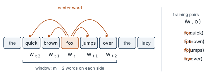
Training pairs. Take the corpus as one token sequence w_1, \dots, w_T. Choose a window half-width m (for example m = 2). For each position t, the center word is w_t and the context words are w_{t+j} for -m \le j \le m, j \ne 0. Each (center, context) pair is one training example. We write a generic pair as (w, o): center word w, context (“outside”) word o.

A sentence of eight tokens with the center word fox highlighted and a window of two words on each side bracketed. Arrows run from fox to quick, brown, jumps and over. Beside the sentence, the four training pairs are listed: (fox, quick), (fox, brown), (fox, jumps), (fox, over). — Figure 1: Skip-gram training pairs. With half-width m = 2, the center word w_t (*fox*) is paired with each of the four words in its window, giving four (center, context) pairs (w, o).

Two vectors per word. Each word gets two embeddings:

e_w \in \mathbb{R}^d, used when w is the center word (row w of E);
u_w \in \mathbb{R}^d, used when w is a context word (row w of a second matrix U \in \mathbb{R}^{|V| \times d}).

The parameters are \theta = \{E, U\}. Two matrices keep the model simple: with a single matrix, the score of a word with itself, e_w^\top e_w, would be large, yet a word rarely appears in its own context. After training we keep E as the word vectors and usually discard U.

The model. The score of a pair is the dot product u_o^\top e_w. A softmax over the vocabulary turns scores into a probability:

P_\theta(o \mid w) = \frac{\exp(u_o^\top e_w)}{\sum_{v \in V} \exp(u_v^\top e_w)} \tag{2}

The loss is the average negative log-likelihood of the observed context words:

\mathcal{L}_{\text{softmax}}(\theta) = -\frac{1}{T} \sum_{t=1}^{T} \sum_{\substack{-m \le j \le m \\ j \ne 0}} \log P_\theta(w_{t+j} \mid w_t) \tag{3}

Why this is too slow. Take one pair (w, o) and differentiate -\log P_\theta(o \mid w) with respect to the center vector. Write -\log P_\theta(o \mid w) = -u_o^\top e_w + \log \sum_{v} \exp(u_v^\top e_w). Then

\frac{\partial}{\partial e_w} \big( -\log P_\theta(o \mid w) \big) = -u_o + \sum_{v \in V} \frac{\exp(u_v^\top e_w)}{\sum_{v'} \exp(u_{v'}^\top e_w)} \, u_v = -u_o + \sum_{v \in V} P_\theta(v \mid w) \, u_v . \tag{4}

The gradient is “observed context vector minus expected context vector”. The expectation is a sum over the whole vocabulary, so every training pair costs O(|V|) and touches every row of U. With billions of pairs and |V| in the hundreds of thousands, this is the bottleneck. Lab: Equation 2 and Equation 3 are the provided function softmax_skipgram_loss, used only to time one training step against SGNS at the lab’s |V| and at |V| = 100{,}000; you do not implement them. Equation 4 is not computed explicitly; autograd applies it in that timing cell.

Check yourself. A text has T = 8 tokens and the window half-width is m = 2, as in Figure 1. How many (center, context) pairs does it produce? With a full softmax and |V| = 100{,}000, how many rows of U does the gradient of one of those pairs touch?

Answer

26 pairs, not 2mT = 32: the windows are cut off at the ends of the text. The eight positions have 2, 3, 4, 4, 4, 4, 3 and 2 context words. Each pair touches all 100,000 rows of U, because the sum in Equation 4 runs over the whole vocabulary: the observed row u_o once, and every row u_v with weight P_\theta(v \mid w). So this 8-token text already costs 2.6 million row updates per pass. That is the cost negative sampling removes.

4. Negative Sampling

Negative sampling (Mikolov et al., 2013) replaces the |V|-way prediction with a much cheaper binary one. This is the derivation the lab implements, so we take it step by step.

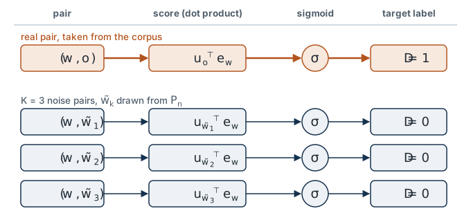
Step 1: change the question. Instead of “which word is in the context of w?”, ask “is the pair (w, o) a real pair from the corpus, or a fake one?” Let D \in \{0, 1\} be that label: D = 1 for a real pair. Model it with logistic regression on the same dot-product score:

P_\theta(D = 1 \mid w, o) = \sigma(u_o^\top e_w), \qquad \sigma(x) = \frac{1}{1 + e^{-x}} \tag{5}

where \sigma is the sigmoid function. Lab: the two score lines of sgns_loss (Exercise 1) compute these dot products for a batch.

Step 2: make fake pairs. A classifier needs negative examples. For each real pair (w, o), draw K negative samples \tilde{w}_1, \dots, \tilde{w}_K from a noise distribution P_n over the vocabulary and treat each (w, \tilde{w}_k) as a fake pair. Mikolov et al. report that K between 5 and 20 works for small corpora and 2 to 5 for large ones. For the noise distribution they found the unigram distribution raised to the power 3/4 to work best:

P_n(v) = \frac{c(v)^{3/4}}{\sum_{v' \in V} c(v')^{3/4}} \tag{6}

where c(v) is the count of word v in the corpus. The exponent flattens the distribution: rare words are drawn more often than their raw frequency, very frequent words less often. The value 3/4 is empirical, not derived. Lab: Equation 6 is the provided function noise_distribution(counts, power=0.75); the training loop draws the K negatives of each pair from it with torch.multinomial.

Step 3: write the likelihood. Treat the K + 1 labels as independent. The real pair should be classified D = 1 and each fake pair D = 0:

\underbrace{\sigma(u_o^\top e_w)}_{\text{real pair is real}} \; \prod_{k=1}^{K} \underbrace{\big(1 - \sigma(u_{\tilde{w}_k}^\top e_w)\big)}_{\text{fake pair is fake}}

Step 4: simplify with 1 - \sigma(x) = \sigma(-x). This identity follows from the definition: 1 - \frac{1}{1 + e^{-x}} = \frac{e^{-x}}{1 + e^{-x}} = \frac{1}{1 + e^{x}} = \sigma(-x). Take the negative log of the likelihood to get the loss for one pair:

\mathcal{L}_{\text{SGNS}}(w, o) = -\log \sigma(u_o^\top e_w) \; - \sum_{k=1}^{K} \log \sigma(-u_{\tilde{w}_k}^\top e_w), \qquad \tilde{w}_k \sim P_n \tag{7}

This is the skip-gram negative-sampling (SGNS) loss. The training loss is its average over all (center, context) pairs in the corpus. The first term pulls e_w and u_o together (large dot product); the second pushes e_w away from the context vectors of random words. Lab: Exercise 1 implements Equation 7 as sgns_loss(e_center, u_context, u_negatives), averaged over a batch.

One value is worth knowing by heart. If every score is 0, then \sigma(0) = \tfrac12 and each of the K + 1 terms is -\log \tfrac12 = \log 2, so \mathcal{L}_{\text{SGNS}} = (K + 1) \log 2, about 4.159 for K = 5. That is the loss of a model that cannot tell real pairs from noise; the Exercise 1 checkpoint tests it, and the lab’s training curve starts there.

Worked example: one real pair, two negatives. Take K = 2 and suppose the current vectors give the scores u_o^\top e_w = 2, u_{\tilde{w}_1}^\top e_w = -1 and u_{\tilde{w}_2}^\top e_w = 0.5. The three terms of Equation 7 are:

Pair	Score	Label D	\sigma(\text{score})	Loss term
real, (w, o)	2	1	0.881	-\log \sigma(2) = 0.127
noise, (w, \tilde{w}_1)	-1	0	0.269	-\log \sigma(1) = 0.313
noise, (w, \tilde{w}_2)	0.5	0	0.622	-\log \sigma(-0.5) = 0.974

So \mathcal{L}_{\text{SGNS}} = 0.127 + 0.313 + 0.974 = 1.414, below the (K + 1)\log 2 = 2.079 of a model that knows nothing. Most of the remaining loss comes from the second noise word: the model gives that fake pair a probability of 0.622 of being real.

Four rows. The first row is the real pair (w, o): its score, u_o transpose e_w, feeds a sigmoid, and the target label is D = 1. The other three rows are noise pairs (w, w-tilde-1) to (w, w-tilde-3): each score, u_w-tilde-k transpose e_w, feeds a sigmoid, and the target label is D = 0. — Figure 2: Negative sampling as binary classification. The real pair (w, o) and K = 3 noise pairs (w, \tilde{w}_k) each pass a dot-product score through a sigmoid. The target label is D = 1 for the real pair and D = 0 for the noise pairs.

Step 5: the gradients. We need one derivative: \frac{d}{dx} \log \sigma(x) = \frac{\sigma'(x)}{\sigma(x)} = 1 - \sigma(x), using \sigma'(x) = \sigma(x)(1 - \sigma(x)). Replacing x by -x and applying the chain rule gives \frac{d}{dx} \log \sigma(-x) = -(1 - \sigma(-x)) = -\sigma(x). Apply the chain rule to each term of Equation 7:

\begin{aligned} \frac{\partial \mathcal{L}_{\text{SGNS}}}{\partial e_w} &= -\big(1 - \sigma(u_o^\top e_w)\big)\, u_o \;+\; \sum_{k=1}^{K} \sigma(u_{\tilde{w}_k}^\top e_w)\, u_{\tilde{w}_k} \\[4pt] \frac{\partial \mathcal{L}_{\text{SGNS}}}{\partial u_o} &= -\big(1 - \sigma(u_o^\top e_w)\big)\, e_w \\[4pt] \frac{\partial \mathcal{L}_{\text{SGNS}}}{\partial u_{\tilde{w}_k}} &= \sigma(u_{\tilde{w}_k}^\top e_w)\, e_w \end{aligned} \tag{8}

(If the same word is drawn twice among the negatives, its gradients add.) Read each line as “prediction error times the other vector”: the error is \sigma(\cdot) - D, the predicted probability minus the label. It is the logistic-regression gradient from Module 1, with the difference that both the “features” and the “weights” are learned.

What we gained. One update now touches K + 2 vectors instead of |V| + 1: the cost per pair drops from O(|V|) to O(K). Lab: the Exercise 1 checkpoint compares autograd’s gradient of your sgns_loss against Equation 8.

What we gave up. Equation 7 is not an approximation of the softmax likelihood Equation 3, and \sigma(u_o^\top e_w) is not a normalized distribution over words. SGNS gives good vectors, not a language model.

Worked example, continued: the gradients. For the three scores above, the prediction errors \sigma(\cdot) - D are 0.881 - 1 = -0.119 for the real pair, 0.269 for the first noise pair and 0.622 for the second. Equation 8 multiplies each by the other side’s vector:

\frac{\partial \mathcal{L}_{\text{SGNS}}}{\partial u_o} = -0.119\, e_w, \qquad \frac{\partial \mathcal{L}_{\text{SGNS}}}{\partial u_{\tilde{w}_1}} = 0.269\, e_w, \qquad \frac{\partial \mathcal{L}_{\text{SGNS}}}{\partial u_{\tilde{w}_2}} = 0.622\, e_w .

Gradient descent subtracts these. So u_o takes a small step toward e_w (the real pair is already scored well), u_{\tilde{w}_1} a moderate step away from it, and u_{\tilde{w}_2} the largest step away, because it is the pair the model currently gets most wrong. The center vector moves by the same three errors applied to the three context vectors: \partial \mathcal{L}_{\text{SGNS}} / \partial e_w = -0.119\, u_o + 0.269\, u_{\tilde{w}_1} + 0.622\, u_{\tilde{w}_2}.

Try it: SGNS updates in two dimensions. Four hand-picked vectors in \mathbb{R}^2: a center vector e_w, the context vector u_o of a real pair, and the context vectors \tilde{u}_1, \tilde{u}_2 of K = 2 noise words. (Here \tilde{u}_k is short for u_{\tilde{w}_k}; the plot labels the four vectors “center e”, “real u”, “noise ũ₁” and “noise ũ₂”.) Each step applies Equation 8 once to all four with plain gradient descent. This is an illustration, not lab data.

Predict first. At the start, \tilde{u}_1 points almost the same way as e_w and \tilde{u}_2 points almost the opposite way. Which of the two moves farther in the first step, and along which direction does each context vector move?

viewof sgdSteps = Inputs.range([0, 40], {value: 0, step: 1, label: "Gradient steps taken"})
viewof eta = Inputs.range([0.05, 1], {value: 0.3, step: 0.05, label: "Learning rate"})

sgnsRun = {
  const sigma = (x) => 1 / (1 + Math.exp(-x));
  const dot = (a, b) => a[0] * b[0] + a[1] * b[1];
  const start = {e: [1.0, 0.2], uo: [-0.3, 1.0], neg: [[0.9, 0.6], [-0.8, -0.5]]};
  let {e, uo, neg} = start;
  for (let s = 0; s < sgdSteps; s++) {
    const go = sigma(dot(uo, e)) - 1;               // error on the real pair: sigma - 1
    const gk = neg.map((u) => sigma(dot(u, e)));    // error on each noise pair: sigma - 0
    const ge = [0, 1].map((i) => go * uo[i] + gk[0] * neg[0][i] + gk[1] * neg[1][i]);
    const e0 = e;                                   // all four gradients use the old vectors
    e = e.map((x, i) => x - eta * ge[i]);
    uo = uo.map((x, i) => x - eta * go * e0[i]);
    neg = neg.map((u, j) => u.map((x, i) => x - eta * gk[j] * e0[i]));
  }
  const loss = -Math.log(sigma(dot(uo, e))) - neg.reduce((a, u) => a + Math.log(sigma(-dot(u, e))), 0);
  const cos = (a, b) => dot(a, b) / (Math.hypot(a[0], a[1]) * Math.hypot(b[0], b[1]));
  return {start, e, uo, neg, loss, cos};
}

{
  const r = sgnsRun;
  const rows = (s) => [
    {x: s.e[0], y: s.e[1], name: "center e", kind: "center"},
    {x: s.uo[0], y: s.uo[1], name: "real u", kind: "real context"},
    {x: s.neg[0][0], y: s.neg[0][1], name: "noise ũ₁", kind: "noise"},
    {x: s.neg[1][0], y: s.neg[1][1], name: "noise ũ₂", kind: "noise"}
  ];
  const chart = Plot.plot({
    width: 440, height: 440, grid: true,
    x: {domain: [-2.6, 2.6], label: "dimension 1"}, y: {domain: [-2.6, 2.6], label: "dimension 2"},
    color: {legend: true, domain: ["center", "real context", "noise"], range: ["var(--demo-ink)", "var(--demo-blue)", "var(--demo-orange)"]},
    marks: [
      Plot.link(rows(r.start), {x1: 0, y1: 0, x2: "x", y2: "y", stroke: "kind", strokeOpacity: 0.35, strokeDasharray: "3 3"}),
      Plot.arrow(rows(r), {x1: 0, y1: 0, x2: "x", y2: "y", stroke: "kind", strokeWidth: 2.5}),
      Plot.text(rows(r), {x: (d) => d.x + 0.32 * d.x / Math.hypot(d.x, d.y), y: (d) => d.y + 0.32 * d.y / Math.hypot(d.x, d.y), text: "name", fontSize: 13})
    ]
  });
  return html`${chart}<p>After ${sgdSteps} steps: loss = ${r.loss.toFixed(3)};
  cosine of the center vector with the real context vector = ${r.cos(r.e, r.uo).toFixed(2)}, with ũ₁ = ${r.cos(r.e, r.neg[0]).toFixed(2)}, with ũ₂ = ${r.cos(r.e, r.neg[1]).toFixed(2)}.</p>`;
}

Solid arrows are the current vectors; dashed lines are where they started. Every context vector moves along \pm e_w, the “other side’s vector” of Equation 8, by an amount set by its prediction error: u_o toward e_w, both noise vectors away, and \tilde{u}_1 much farther than \tilde{u}_2 because its error is larger (0.74 against 0.29 at the start). The center vector turns toward u_o and away from the noise. Keep stepping and the loss falls toward 0 while the vectors keep growing: with one pair and two fixed negatives nothing stops the model from becoming ever more confident. In real training each vector is pulled by many pairs and fresh negatives at once.

Check yourself. Two words have counts c = 1{,}000 and c = 10. Under the raw unigram distribution the frequent word is drawn 100 times as often as the rare one. How many times as often under the noise distribution Equation 6? What would an exponent of 0 do?

Answer

The ratio becomes (1000/10)^{3/4} = 100^{0.75} \approx 31.6. The normalizing sum cancels in a ratio, so only the exponent matters. The rare word is still drawn less often, but relative to the frequent word about three times more often than the raw counts would give. An exponent of 0 gives every word the same probability 1/|V|: negatives would then be mostly rare words, since most of the vocabulary is rare (Zipf’s law), and frequent words would almost never be pushed away from anything. The value 3/4 sits between the two extremes and was chosen by experiment.

Check yourself. A colleague trains SGNS and wants to report its perplexity on held-out text, to compare with Module 1’s bigram model. What do you tell them?

Answer

It cannot be done. Perplexity needs a normalized next-token distribution P(w_t \mid w_{<t}). SGNS produces \sigma(u_o^\top e_w), the probability that one pair is real; summed over all o in the vocabulary these values do not add up to 1, and nothing in Equation 7 pushes them to. SGNS also predicts words on both sides of the center, not the next word from the previous ones. Negative sampling is a different objective from the softmax, not a faster way to compute it. To get a perplexity you need a model with a softmax over the vocabulary, such as the one in section 8.

Optional: Subsampling Frequent Words, and the Dynamic Window

Words such as the appear in almost every window and say little about their neighbors. Mikolov et al. (2013) discard each occurrence of word v before building pairs with probability

P_{\text{discard}}(v) = 1 - \sqrt{\frac{\tau}{f(v)}} \tag{9}

(taken as 0 when negative), where f(v) = c(v) / T is the relative frequency of v and \tau is a threshold, typically around 10^{-5} for very large corpora. This speeds up training and improves the vectors of rare words. The lab uses \tau = 10^{-3}, a larger value suited to its corpus of about one million tokens, and draws a fresh subsample every epoch.

word2vec also uses a dynamic window: for each center word it draws a width b uniformly from 1, \dots, m and pairs the center only with words within b positions. A context word j positions away is used with probability (m - j + 1)/m, so near neighbors count more than far ones. The lab does the same, with m = 5, and never lets a window cross from one abstract into the next. Lab: Equation 9 and the dynamic window are in the provided function make_pairs.

Optional: What SGNS Is Really Computing

Levy and Goldberg (2014) showed that, with enough dimensions, the SGNS optimum satisfies

u_o^\top e_w = \mathrm{PMI}(w, o) - \log K, \qquad \mathrm{PMI}(w, o) = \log \frac{P(w, o)}{P(w)\,P(o)}

where PMI is the pointwise mutual information of the pair, estimated from co-occurrence counts. So SGNS implicitly factorizes a shifted PMI matrix. This connects word2vec back to the count-based methods of Module 1: the neural model is a compact, weighted factorization of a count matrix, not a different kind of object.

5. CBOW and GloVe in Brief

CBOW (continuous bag of words) is skip-gram reversed. It averages the embeddings of the context words and predicts the center word from that average. It trains faster, because there is one prediction per window rather than 2m; skip-gram tends to do better on rare words.

GloVe (Global Vectors; Pennington et al., 2014) starts from global counts rather than a stream of windows. Let c(w, o) be the number of times o occurs in the context of w over the whole corpus. GloVe fits the vectors by weighted least squares so that dot products match log counts:

\mathcal{L}_{\text{GloVe}} = \sum_{w, o \,:\, c(w,o) > 0} f\big(c(w, o)\big) \, \big( e_w^\top u_o + b_w + \tilde{b}_o - \log c(w, o) \big)^2 \tag{10}

where b_w and \tilde{b}_o are per-word scalar biases and f is a weighting function that grows as (x / x_{\max})^{3/4} and is capped at 1 for x \ge x_{\max}, so that rare pairs count for less and very frequent pairs do not dominate. Skip-gram and GloVe use the same co-occurrence information and, with comparable tuning, give vectors of similar quality (Levy, Goldberg and Dagan, 2015). Lab: the stretch section loads pretrained GloVe vectors; you do not train Equation 10.

Analogies. Trained embeddings show approximately linear structure: the offset e_{\text{king}} - e_{\text{man}} is close to e_{\text{queen}} - e_{\text{woman}}. An analogy “a is to b as a' is to ?” is answered by

\arg\max_{v \in V \setminus \{a, b, a'\}} \cos\big(e_v, \; e_b - e_a + e_{a'}\big) \tag{11}

Note the excluded set: without it the answer is usually one of the three input words. Lab: Equation 11 is the provided function analogy(a, b, a2, E), which calls your Exercise 2 function nearest_neighbors on the vector e_b - e_a + e_{a'} with the three inputs excluded.

How much of this structure appears depends on the data. Lab 2 trains on about one million tokens of arXiv abstracts and scores its vectors on 20 analogies fixed before training; its stretch section repeats the test with pretrained GloVe vectors, trained on about 6 billion tokens. Lab: Section A3 also draws a two-dimensional PCA picture of 60 of your embeddings, from four topic groups chosen before training. The results are in the box after the lab, below.

After the Lab: What Lab 2 Measured in Section A3

Open this after Section A3 of the lab (and its stretch section, for GloVe), so that it does not answer the lab’s predictions for you. There, 4 of 20 analogies fixed before training come out right (0.20), mostly word forms such as dataset : datasets. The same lists answered with pretrained GloVe vectors, trained on about 6 billion tokens, score 11 of the 19 that GloVe can attempt (0.58), against 4 of the same 19 (0.21) for the lab’s vectors. That comparison changes the objective as well as the data, but controlled comparisons find that the choice between SGNS and GloVe matters less than hyperparameters and data (Levy, Goldberg and Dagan, 2015). The amount of data is the likely limit, not the objective.

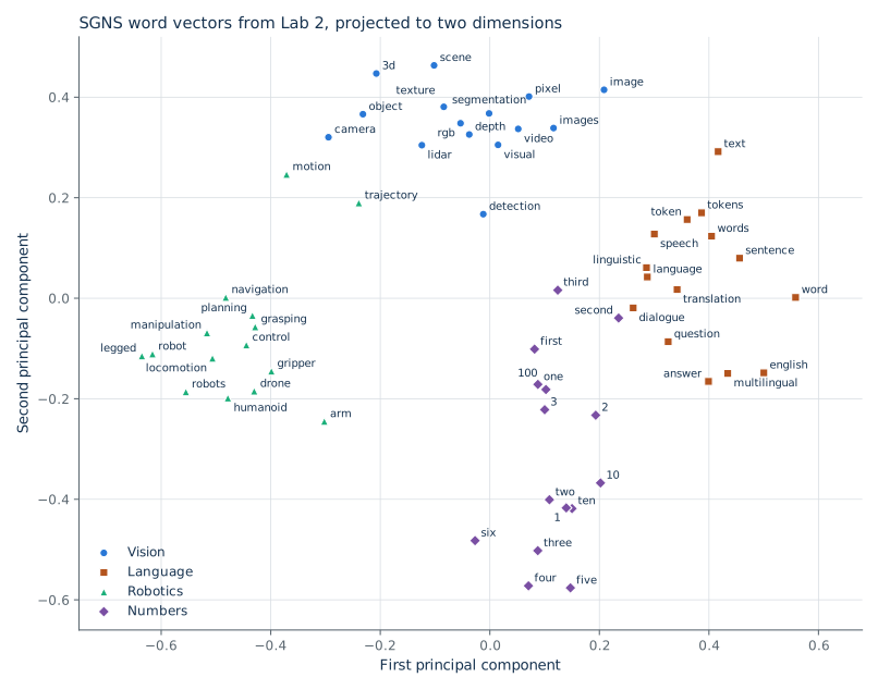
Figure 3: Lab 2’s SGNS word vectors for 60 words, chosen before training from four groups and projected to two dimensions by principal component analysis (PCA). The vectors were scaled to unit length and centered first, so the plot shows directions, as cosine similarity sees them. Each group has its own color and marker. Two dimensions keep only part of the variance; a word that looks misplaced may be far away along a direction not shown.

The picture is cleaner than the analogies: words from papers on the same topic are close, which is what the distributional hypothesis predicts. Lab: Section A3 draws this plot from your embeddings and saves the coordinates; Figure 3 is drawn from the recorded run (scripts/make_figures_02.py).

Check yourself. Suppose the offset idea holds only loosely: e_b - e_a is a short vector compared with e_{a'} itself. Remove the exclusion set from Equation 11, so that the arg max runs over all of V. Which word will the analogy “a is to b as a' is to ?” most likely return?

Answer

Most likely a' itself. The query vector is e_{a'} + (e_b - e_a): the vector of a' plus a small displacement. Unless the displacement is large, the vector with the highest cosine to “e_{a'} plus a little” is e_{a'}. So without the exclusion the method mostly returns one of its own inputs, and the reported accuracy of the analogy test depends on the exclusion rule. That is one reason to read analogy scores as evidence of some linear structure, not as a test of whether the model understands the relation.

6. PyTorch Refresher

Everything from here to Module 12 is written in PyTorch. Four ideas are enough for today.

Tensors are arrays that live on a device (CPU or GPU) and may record the operations applied to them.
Autograd. If a tensor has requires_grad=True, calling .backward() on a scalar computed from it fills in .grad with the derivative. We write the loss; PyTorch applies the chain rule.
nn.Module bundles parameters with a forward method. nn.Embedding(V, d) holds the matrix E and returns rows of it; nn.Linear(a, b) holds a weight matrix and a bias.
The training loop is always the same five lines.

import torch, torch.nn as nn

class SkipGram(nn.Module):
    def __init__(self, vocab_size, d):
        super().__init__()
        self.E = nn.Embedding(vocab_size, d)   # center vectors  e_w
        self.U = nn.Embedding(vocab_size, d)   # context vectors u_w
        nn.init.uniform_(self.E.weight, -0.5 / d, 0.5 / d)   # word2vec's initialization:
        nn.init.zeros_(self.U.weight)                        # E small and random, U zero

    def forward(self, center, context, negatives):
        # center, context: (B,)   negatives: (B, K)
        return sgns_loss(self.E(center), self.U(context), self.U(negatives))

model = SkipGram(vocab_size=12_470, d=100)   # Lab 2: 12,469 words plus <pad>
opt = torch.optim.Adam(model.parameters(), lr=1e-2)

for center, context, negatives in loader:          # 1. get a batch
    loss = model(center, context, negatives)       # 2. forward pass: compute the loss
    opt.zero_grad()                                # 3. clear old gradients
    loss.backward()                                # 4. backward pass: autograd
    opt.step()                                     # 5. update the parameters

B is the batch size. The function sgns_loss is Equation 7 averaged over the batch: the one piece you write in Exercise 1. Step 4 computes Equation 8 for you; the gradient is nonzero only in the rows of E and U that the batch used. loader stands for whatever yields batches: in the lab it is a loop over the shuffled pairs from make_pairs, 16,384 pairs at a time, with the negatives drawn from P_n inside the loop.

The two nn.init lines are word2vec’s initialization, and the lab uses them too. With U = 0 every score u^\top e is 0 at the first step, so the first loss is exactly (K + 1)\log 2; the lab asserts this. At that first step only U moves: in Equation 8 the gradient with respect to e_w is a weighted sum of context vectors, and all of them are still zero.

Check yourself. To simplify the code, someone initializes both E and U to zero. Use Equation 8 to predict the loss after 1,000 training steps.

Answer

It is still (K + 1)\log 2, the starting value. Every gradient in Equation 8 is an error times the other side’s vector. The gradient for e_w is a weighted sum of context vectors, all zero. The gradients for u_o and u_{\tilde{w}_k} are multiples of e_w, also zero. Nothing moves at step 1, so nothing moves at step 2, and so on: zero is a stationary point of the loss, and the optimizer never leaves it. One of the two matrices must start nonzero to break the tie. That is why word2vec, and the lab, start E small and random and only U at zero.

7. Feed-Forward Networks and Backpropagation

Embeddings give us features. To use them for classification we need a model on top. Module 1’s classifier was linear in its input; a feed-forward network adds one nonlinear layer.

From words to a document vector. A document is a token sequence w_1, \dots, w_T. The simplest fixed-size representation is the average of its word embeddings:

x = \frac{1}{T} \sum_{t=1}^{T} e_{w_t} \; \in \mathbb{R}^d \tag{12}

This replaces Module 1’s TF-IDF vector in \mathbb{R}^{|V|} with a dense vector in \mathbb{R}^d. Lab: Exercise 3 implements Equation 12 as average_embeddings(token_ids, mask, E) for a padded batch: mask is 1 at real tokens and 0 at padding, so the sum and the count T run over real tokens only. Words outside the vocabulary are dropped before averaging, and a provided cell standardizes the features with the training split’s mean and standard deviation.

The network. With input x, label y \in \{1, \dots, C\} and C classes:

\begin{aligned} h &= \mathrm{ReLU}(W_1 x + b_1) && W_1 \in \mathbb{R}^{d_h \times d},\; b_1 \in \mathbb{R}^{d_h} \\ z &= W_2 h + b_2 && W_2 \in \mathbb{R}^{C \times d_h},\; b_2 \in \mathbb{R}^{C} \\ \hat{y} &= \mathrm{softmax}(z) && \hat{y}_i = \frac{\exp(z_i)}{\sum_{j=1}^{C} \exp(z_j)} \\ \mathcal{L} &= -\log \hat{y}_y \end{aligned} \tag{13}

Here h is the hidden vector with d_h units, \mathrm{ReLU}(a) = \max(0, a) applied elementwise, z are the logits, \hat{y} the predicted class probabilities and \mathcal{L} the cross-entropy loss. Without the ReLU, the two layers would collapse into one linear map and we would be back at logistic regression. Lab: Exercise 4 implements the forward pass of Equation 13 as FeedForwardClassifier.forward.

Backpropagation is the chain rule applied from the loss backwards, reusing each intermediate result. At the logits the error is \hat{y} - \mathrm{onehot}(y), where \mathrm{onehot}(y) \in \mathbb{R}^C is the one-hot vector of the label: the same “prediction minus target” form as Equation 4 and Equation 8. Each earlier layer multiplies the error arriving from above by its own local derivative (Equation 14, in the optional box). Lab: you do not write Equation 14; loss.backward() computes it. A provided cell checks autograd’s \partial \mathcal{L} / \partial z against \hat{y} - \mathrm{onehot}(y).

The chain rule does not stop at x: through Equation 12 it reaches every embedding in the document, so embeddings can be trained by the classification loss too. In the lab’s core path they stay frozen, so that the comparison with TF-IDF measures the features and nothing else.

Optional: Backpropagation Through the Network, Line by Line

Let \mathrm{onehot}(y) \in \mathbb{R}^C be the one-hot vector of the label, a = W_1 x + b_1 the hidden pre-activation, and \delta denote the gradient of \mathcal{L} with respect to a layer’s pre-activation.

\begin{aligned} \delta_z &= \frac{\partial \mathcal{L}}{\partial z} = \hat{y} - \mathrm{onehot}(y) \\[2pt] \frac{\partial \mathcal{L}}{\partial W_2} &= \delta_z \, h^\top, \qquad \frac{\partial \mathcal{L}}{\partial b_2} = \delta_z \\[2pt] \delta_a &= \big(W_2^\top \delta_z\big) \odot \mathbf{1}[a > 0] \\[2pt] \frac{\partial \mathcal{L}}{\partial W_1} &= \delta_a \, x^\top, \qquad \frac{\partial \mathcal{L}}{\partial b_1} = \delta_a \end{aligned} \tag{14}

where \odot is the elementwise product and \mathbf{1}[a > 0] is 1 where the hidden unit was active and 0 elsewhere (the derivative of ReLU). The first line comes from differentiating \mathcal{L} = -z_y + \log \sum_j \exp(z_j): the derivative with respect to z_i is \hat{y}_i, minus 1 when i = y. It has the same “prediction minus target” form as Equation 4 and Equation 8. Each later line multiplies the error arriving from above by the local derivative of one layer.

One more step of the chain rule gives \partial \mathcal{L} / \partial x = W_1^\top \delta_a, and through Equation 12 a gradient for every embedding in the document.

Check yourself. For one training example, hidden unit 3 has pre-activation a_3 = -0.7. What gradient does this example send to row 3 of W_1 and to entry 3 of b_1? What if a_3 < 0 for every training example?

Answer

Zero, for both. In Equation 14, \delta_a = (W_2^\top \delta_z) \odot \mathbf{1}[a > 0], and the indicator is 0 for unit 3, so entry 3 of \delta_a is 0 whatever error arrives from above. Row 3 of \partial \mathcal{L} / \partial W_1 = \delta_a x^\top is then a zero row. The unit output 0 in the forward pass, so it had no effect on the loss, and it gets no signal. If a_3 < 0 for every example, the unit never receives a gradient and its weights never change again: a “dead” ReLU unit. It is one reason for careful initialization and moderate learning rates.

After the Lab: What Lab 2 Measured

Open this after the lab’s comparison of the two classifiers, so that it does not answer the lab’s prediction for you. Lab 2 trains SGNS embeddings on the text of the 4,800 training abstracts (1,091,692 tokens, labels ignored), then classifies the same 1,600 test abstracts as Lab 1. These are the values recorded in data/baselines.json, measured on a CPU; your run will differ slightly.

Features + model	Dimensions	Test accuracy	Test macro-F1
TF-IDF + logistic regression (Lab 1, `C` = 10)	12,469	0.884	0.884
Averaged SGNS embeddings, frozen, + feed-forward network	100	0.867	0.867
Averaged pretrained GloVe, frozen, + feed-forward network (stretch)	100	0.805	0.805

TF-IDF wins by 27 of the 1,600 papers. In four runs with different random streams the SGNS row ranged from 0.864 to 0.872 accuracy, so the gap is larger than the run-to-run noise. Two readings:

Averaging costs something. A topic is often signaled by a few rare, specific words. TF-IDF gives each its own weight; the average dilutes them among the 227 tokens of an average abstract. With 4,800 labeled papers, a linear model can learn a weight for most useful words directly.
For features, the domain of the training text matters. GloVe was trained on about 5,000 times more text than our SGNS run, but general text: it lacks 8% of the lab’s vocabulary words, many of them telling ones (llms, pretrained), and gives the rest their general-English sense. It scores six points below the in-domain embeddings.

In this comparison more text did not help unless it was text about the task.

8. Bengio’s Neural Language Model

We now have what is needed to repair the n-gram language model. Bengio et al. (2003) keep the n-gram assumption, that the next word depends on the previous n - 1 words, but replace the count table with a feed-forward network over embeddings.

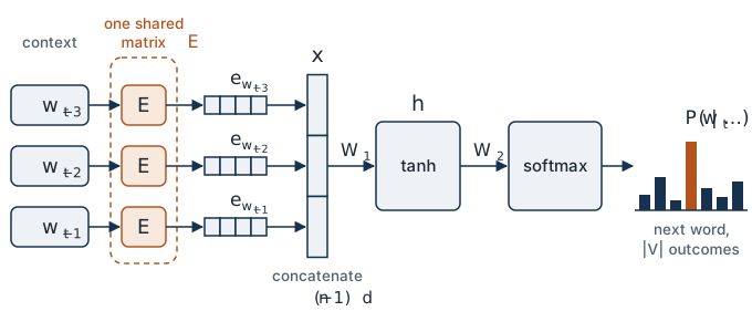
Concatenate the embeddings of the n - 1 context words, pass them through one hidden layer, and take a softmax over the vocabulary:

\begin{aligned} x &= [\, e_{w_{t-n+1}} ; \dots ; e_{w_{t-1}} \,] \in \mathbb{R}^{(n-1)d} \\ h &= \tanh(W_1 x + b_1) \\ P_\theta(w_t \mid w_{t-n+1}, \dots, w_{t-1}) &= \mathrm{softmax}(W_2 h + b_2)_{w_t} \end{aligned} \tag{15}

with W_1 \in \mathbb{R}^{d_h \times (n-1)d} and W_2 \in \mathbb{R}^{|V| \times d_h}. The loss is the average negative log-likelihood of the next word, and its exponential is the perplexity from Module 1, \mathrm{PPL} = \exp\big(-\tfrac{1}{T} \sum_t \log P_\theta(w_t \mid w_{<t})\big), so the two kinds of model can be compared directly.

Left to right: three context words, w_{t-3}, w_{t-2} and w_{t-1}, are each looked up in the same shared embedding matrix E. The three embeddings are concatenated into one vector x, which passes through weights W_1 and a tanh hidden layer h, then through weights W_2 and a softmax, giving a bar chart of the next-word distribution over the vocabulary. — Figure 4: Bengio’s neural language model with n - 1 = 3 context words. Every position looks up its word in the same embedding matrix E. The three embeddings are concatenated into x, a tanh hidden layer gives h, and a softmax over |V| gives the next-word distribution.

This addresses both failures from section 1:

Sparsity. The parameter count is |V| d + d_h (n-1) d + |V| d_h plus biases: linear in |V| and in n, where the n-gram table has |V|^n cells.
Unrelated symbols. If cat and dog have similar embeddings, a context containing dog produces nearly the same x, hence nearly the same prediction, as one containing cat. Probability mass reaches unseen n-grams through similarity, not through a smoothing constant.

The embeddings here are learned by the language-modeling loss itself. Word2vec, ten years later, kept the embedding table and removed the hidden layer and the full softmax to make training on billions of words practical. Lab: Equation 15 is not implemented in Lab 2. Module 3’s lab trains a neural language model and compares its perplexity with the n-gram baseline.

Optional: Details of the Original Model

The model in Bengio et al. (2003) also has optional direct connections from x to the output layer, omitted in Equation 15. Its output softmax has the same O(|V|) cost per example as Equation 2; that cost is what later work, including hierarchical softmax and negative sampling, set out to reduce.

What is still missing. Both models in this module use a fixed, small amount of context, and neither handles word order well:

Averaging (Equation 12) is a bag of words. “The dog bit the man” and “the man bit the dog” get the same vector.
The neural language model sees exactly n - 1 words. A dependency longer than the window is invisible, and widening the window grows W_1 and gives every position its own separate weights.
Each word has one vector regardless of context: bank is the same in “river bank” and “bank account”.

Module 3 takes up the first two: recurrent networks read a sequence of any length in order, carrying a hidden state h_t from one token to the next. The third waits for contextual representations in Modules 5 and 6.

Check yourself. A neural language model (Equation 15) has |V| = 10{,}000, d = 100, d_h = 200 and reads n - 1 = 3 context words. Count its weights, ignoring biases. How many cells does the corresponding 4-gram count table have? Then widen the context to 10 words: how many weights are added, and what does the model still not share?

Answer

Embeddings |V| d = 1{,}000{,}000; hidden layer d_h (n-1) d = 200 \times 300 = 60{,}000; output layer |V| d_h = 2{,}000{,}000. Total: 3.06 million weights, against |V|^4 = 10^{16} cells in the 4-gram table. Widening to 10 context words grows only W_1, from 200 \times 300 to 200 \times 1{,}000: 140,000 more weights. That is cheap, but each of the 10 positions gets its own block of columns in W_1. What the model learns about a word three positions back does not transfer to the same word four positions back, and no fixed width covers every dependency. Sharing one set of weights across positions is the idea of Module 3.

Equations and Where You Implement Them

Function names and signatures are those of the notebook as built.

Equation	What it is	In Lab 2
Equation 1	Cosine similarity	Exercise 2: `nearest_neighbors(query, E, k=10, exclude=(), words=None)`; `query` is a word or a vector
Equation 2, Equation 3	Full-softmax skip-gram	Provided: `softmax_skipgram_loss`, timing comparison only
Equation 4	Full-softmax gradient	Not written; autograd computes it in the timing cell
Equation 5	Real-or-fake pair score	Exercise 1: the two score lines of `sgns_loss`
Equation 6	Noise distribution	Provided: `noise_distribution(counts, power=0.75)`; negatives drawn with `torch.multinomial`
Equation 7	SGNS loss	Exercise 1: `sgns_loss(e_center, u_context, u_negatives)`; Checkpoint 1 tests (K + 1)\log 2 at zero vectors and a hand-computed batch
Equation 8	SGNS gradients	Checkpoint 1 compares autograd with all three lines (divided by B for the batch mean)
Equation 9	Subsampling (optional)	Provided: `make_pairs`, \tau = 10^{-3}, with the dynamic window
Equation 10	GloVe objective	Not trained; the stretch section loads pretrained GloVe vectors
Equation 11	Analogy by vector offset	Provided: `analogy(a, b, a2, E)`, built on `nearest_neighbors`
Figure 3	PCA of 60 embeddings	Provided plot in Section A3; coordinates saved to `lab02_pca_points.csv`
Equation 12	Averaged embeddings	Exercise 3: `average_embeddings(token_ids, mask, E)`; Checkpoint 3 tests padding and the empty document
Equation 13	Feed-forward classifier	Exercise 4: `FeedForwardClassifier.forward`; trained by the provided `train_classifier`
Equation 14	Backpropagation	Provided cell checks autograd’s \partial \mathcal{L} / \partial z against \hat{y} - \mathrm{onehot}(y); otherwise `loss.backward()`
Equation 15	Neural language model	Not in Lab 2; Module 3
Levy–Goldberg PMI identity	What SGNS computes (optional)	Not in the lab

Summary

Count-based models fail on sparsity and on treating words as unrelated symbols. Dense embeddings e_w \in \mathbb{R}^d address both.
The distributional hypothesis supplies the training signal: predict a word’s neighbors.
Skip-gram with a full softmax costs O(|V|) per pair. Negative sampling replaces it with K + 1 binary classifications, giving the loss Equation 7 at cost O(K).
Every gradient in this module has the form “prediction minus target, times the other side’s vector”.
A feed-forward network over averaged embeddings is a dense replacement for TF-IDF plus a linear classifier. It uses 100 dimensions instead of 12,469. Whether it is more accurate is an empirical question, which Lab 2 answers on its test split (the box after the lab in section 7).
The amount and the domain of the training text shape what embeddings are good for. Lab 2 compares its own vectors with pretrained GloVe, trained on far more but general text, on analogies and as classifier features (the boxes after the lab in sections 5 and 7).
Bengio’s neural language model applies the same pieces to next-word prediction and generalizes to unseen n-grams through embedding similarity.
Open problem for Module 3: order and long-range dependence.

Gotchas and Troubleshooting

“Negative sampling is a fast approximation of the softmax.” It is a different objective. It does not yield normalized probabilities P_\theta(o \mid w) and cannot be used to compute perplexity.
“Similar vectors mean synonyms.” Cosine similarity reflects shared contexts. Antonyms (hot, cold) and co-hyponyms (Tuesday, Friday) share contexts and end up close.
“The analogy trick shows the model understands relations.” The result depends on excluding the input words in Equation 11 and on the corpus. On a small corpus most analogies fail, and controlled comparisons find that the choice between SGNS and GloVe matters less than hyperparameters and data (Levy, Goldberg and Dagan, 2015). Lab 2 counts how many succeed with its own vectors and with GloVe (the box after the lab in section 5).
“An embedding layer is a special kind of layer.” It is a linear layer applied to a one-hot vector, implemented as a row lookup.
“Dense embeddings must beat TF-IDF.” Averaging discards word order and blurs distinctive words. On topic classification with plenty of labeled data, TF-IDF with a linear model is a strong baseline. Measure before claiming: Lab 2 does, and its result is in the box after the lab in section 7.
“Each word has one meaning, so one vector is enough.” Static embeddings merge all senses of a word into one point. That limitation motivates the contextual models of Day 2.