Sequence Models

Day 1 · Foundations Module 3 95 minutes (45 briefing, 50 lab) 13:35 briefing · 14:20 lab

RNNs, LSTMs and neural language modeling, and why gradients vanish over long sequences.

Open the lab in Colab PyTorch

Duration: 95 minutes (45 briefing, 50 lab)
Level: 200 · Intermediate
Lab runtime: Google Colab, free T4 GPU · about 10 minutes of compute
Accounts and cost: Google. Free
Without API keys: the lab always runs its real models

What You Will Build

In this module you will:

Implement the RNN and LSTM cell updates and the language-model loss
Explain vanishing gradients and how gating addresses them, from measured gradient decay
Evaluate the LSTM against the n-gram baseline in a like-for-like perplexity comparison

New terms, in the glossary: recurrent neural network (RNN), teacher forcing, long short-term memory (LSTM).

Before You Start

Module 2 · Word Vectors and Neural Networks and its lab, and the modules before it: this module measures its results against theirs.
A Google account, and the Colab runtime set to T4 GPU (Runtime → Change runtime type).
No API keys: the lab runs its own models throughout.

Where we are. Module 2 gave words vectors, and with them a language model that generalizes across similar words. But that model reads a fixed window of n - 1 tokens with separate weights for each position, and the averaged-embedding classifier ignores order altogether. This module asks one question: can a single set of weights read a sequence of any length, in order, and still learn what happened many steps back?

In the Lab

Open the lab in Colab

5 exercises in 5 parts. The notebook budgets 37 minutes for them; the lab slot is 50 minutes. Each exercise you write is a # TODO stub with a folded solution beneath it and a checkpoint that passes or fails; where people tend to stall, a folded hint sits above the stub.

Task	Briefing section	Time
Part A · Recurrent Networks
Exercise 1 · An RNN Cell by Hand	2	8 min
Exercise 2 · Loss, Perplexity and Bits per Character	3, 6	6 min
Exercise 3 · Vanishing and Exploding Gradients	4	9 min
Part B · The LSTM
Exercise 4 · The LSTM Cell	5	6 min
Part C · Generating Text
Exercise 5 · Sampling With Temperature	7 (Reference)	8 min

Challenge · Top-k and Nucleus Sampling

Optional, for anyone who finishes the core path early: the notebook’s stretch section, after the last checkpoint.

When you are done. Runtime → Disconnect and delete runtime releases the machine; your keys stay in Colab Secrets for the next lab.

Agenda

Minutes	Section	In the room
0–2	1. Where Module 2 Left Us	—
2–5	2. The Recurrent Neural Network	—
5–13	3. The RNN Language Model	—
13–27	4. Backpropagation Through Time	Demo (4 min)
27–39	5. The LSTM	Check yourself (2 min)
39–45	6. Measuring the Improvement Fairly	Check yourself (2 min)
45	Total	37 minutes of exposition, 8 of activities

Checks, demos and predictions listed here are part of the live session and its minutes; the others on the page are for reading afterwards.

Read now · Sections 1–6, in the agenda above.

Use in the lab · Exercise 1: section 2; Exercise 2: sections 3 and 6; Exercise 3: section 4; Exercise 4: section 5; Exercise 5: section 7 (section 7: Reference; the exercise restates what it needs).

Read later · Section 7, Generating Text: Sampling Strategies (Reference); the collapsed callouts marked After the Lab; Further Reading.

In section 4 the demo plays out the same one-unit RNN, and the same three cases, as the worked example before it. In the room, use the demo in place of walking through the example’s table, which stays on the page for reading.

1. Where Module 2 Left Us

Both neural models of Module 2 have the same blind spot.

The fixed-window neural language model (Bengio et al.) predicts the next token from the previous n-1 tokens. It shares statistical strength between similar words, which the n-gram model of Module 1 could not, but it still sees nothing beyond the window. Widening the window adds a new block of weights for each position, and what the model learns about a word at position 3 does not transfer to the same word at position 4.
Averaged embeddings discard order completely: “dog bites man” and “man bites dog” get the same vector.

Language has dependencies of no fixed length. In “The keys to the cabinet in the hall are missing”, the verb are agrees with keys, seven words earlier. In a play, the speaker of a line is decided by a name several hundred characters earlier.

We want a model that (1) reads a sequence of any length, (2) applies the same parameters at every position, and (3) carries what it has read forward in a state. That model is the recurrent neural network (RNN).

Notation for This Module

The workshop notation applies. Tokens are w_1,\dots,w_T, with T the sequence length, drawn from a vocabulary V of size |V|. In this module’s lab the tokens are characters, so |V| is small: the 65 distinct characters of the training split.

Symbol	Meaning
x_t = e_{w_t} \in \mathbb{R}^d	input vector at step t: the embedding of token w_t, dimension d
h_t \in \mathbb{R}^{d_h}	hidden state after reading w_1,\dots,w_t; d_h is the hidden size; h_0 = 0
a_t \in \mathbb{R}^{d_h}	pre-activation at step t, so that h_t = \tanh(a_t)
W, U, b	recurrent (hidden-to-hidden) matrix, input-to-hidden matrix, bias
W_o, b_o	output matrix (\|V\| \times d_h) and output bias
z_t \in \mathbb{R}^{\|V\|}, \hat{y}_t = \mathrm{softmax}(z_t)	logits and predicted distribution over the next token
\mathcal{L}_t, \mathcal{L}	loss at step t, and its mean over the sequence
\theta	all parameters
\sigma	the logistic sigmoid, applied elementwise
\odot	elementwise product
\tau	sampling temperature (not T, which is sequence length)

Notation Clashes, Resolved

Module 1 uses c(\cdot) for a count, as in c(w_{t-1}, w_t). The LSTM literature uses c_t for the cell state. In this module c_t with a time subscript is always the LSTM cell state, a vector in \mathbb{R}^{d_h}. The count function is always written with an argument in parentheses, c(\cdot), and appears only where we describe the n-gram baseline.

Three letters from Module 2 also change meaning here.

U is the input-to-hidden matrix, (d_h, d), not Module 2’s matrix of context vectors.
\tau is the sampling temperature (section 7), not Module 2’s subsampling threshold. From here on, plain \tau is always a temperature.
o_t is the LSTM’s output gate (section 5), not Module 2’s context word o.

2. The Recurrent Neural Network

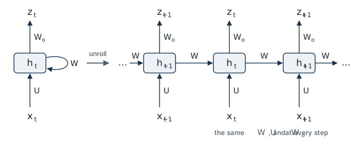
An RNN reads one token at a time and updates a state vector with the same function at every step:

a_t = W h_{t-1} + U x_t + b, \qquad h_t = \tanh(a_t). \tag{1}

Every symbol is in the table above. The two things to notice are that W, U and b carry no time index (the parameters are shared across positions) and that h_t depends on h_{t-1}, which depends on h_{t-2}, and so on. So h_t is a function of the whole prefix w_1,\dots,w_t, with no window.

An RNN drawn as a loop and unrolled over three time steps with shared weights. — Figure 1: An RNN drawn as a loop (left) and unrolled over three time steps (right). Inputs x_t enter through U, hidden states h_t pass to the next step through W, and logits z_t leave through W_o. The same W, U and W_o are used at every step.

In code, one step is two lines. Shapes are for a batch of B sequences.

def rnn_cell_step(x_t, h_prev, W, U, b):
    # x_t: (B, d)   h_prev: (B, d_h)   W: (d_h, d_h)   U: (d_h, d)   b: (d_h,)
    a_t = h_prev @ W.T + x_t @ U.T + b      # (B, d_h)
    return torch.tanh(a_t)                   # h_t: (B, d_h)

In the lab: Exercise 1 asks you to write rnn_cell_step, which is Equation 1. The checkpoint compares your output with PyTorch’s nn.RNNCell given the same weights.

Check yourself. The lab’s RNN has d = 64 and d_h = 256. How many parameters do W, U and b of Equation 1 hold? How does that number change if the model must read 1,000 characters of context instead of 128? Compare with the fixed-window model of Module 2 at the same sizes.

Answer

W has 256 \times 256 = 65{,}536 entries, U has 256 \times 64 = 16{,}384 and b has 256: 82,176 in total. The number does not change with the length of the sequence, because the same three objects are applied at every step. A fixed-window model concatenates the context embeddings, so each extra position of context adds a block of d_h \times d = 16{,}384 weights to its hidden layer, and those weights are trained only on what appears at that one position. The RNN pays for long context in computation and in how hard it is to train, not in parameters.

3. The RNN Language Model

A language model assigns a probability to the next token given the tokens so far. With an RNN, the hidden state is the summary of “the tokens so far”:

z_t = W_o h_t + b_o, \qquad \hat{y}_t = \mathrm{softmax}(z_t), \qquad P_\theta(w_{t+1} \mid w_1,\dots,w_t) = \hat{y}_t[w_{t+1}], \tag{2}

where \hat{y}_t[w] is the entry of \hat{y}_t for token w. Compare this with Module 1’s bigram model, which conditions on w_t alone, and with Bengio’s model, which conditions on a fixed window.

The loss is the same cross-entropy as in Modules 1 and 2, now averaged over the positions of a sequence:

\mathcal{L}_t = -\log \hat{y}_t[w_{t+1}], \qquad \mathcal{L} = \frac{1}{T}\sum_{t=1}^{T} \mathcal{L}_t. \tag{3}

Here the model reads w_1,\dots,w_T and the targets are w_2,\dots,w_{T+1}: the same text shifted by one position.

Perplexity is the exponential of this mean loss, exactly as defined in Module 1 with the natural logarithm:

\mathrm{PPL} = \exp(\mathcal{L}) = \exp\Big(-\frac{1}{T}\sum_{t} \log P_\theta(w_{t+1} \mid w_1,\dots,w_t)\Big). \tag{4}

In the lab: Exercise 2 asks you to write lm_loss_and_ppl(logits, targets), which is Equation 3 and Equation 4. It returns the mean loss in nats, the perplexity and the bits per character (defined in the section on measuring fairly). The checkpoint feeds it equal logits, for which the perplexity must equal |V| = 65, and compares the loss with F.cross_entropy. The same function is the training loss and scores every model in the lab, the n-gram baseline included.

Teacher Forcing

During training, the input at step t is the true token w_t from the corpus, whatever the model predicted at step t-1. This is called teacher forcing. It has two consequences.

All T losses of a sequence come from one forward pass, because the inputs are known in advance.
At generation time there is no teacher: the model reads its own samples. It can drift into prefixes it never saw in training, and errors can compound. This mismatch is called exposure bias. We accept it here; it is one reason sampling choices (the last section) matter.

Training on a Long Text: Truncated Backpropagation

The corpus is one long string, far too long to treat as a single sequence. At each training step the lab takes 64 random chunks of T = 128 characters from the training split, runs the model on each from h_0 = 0, computes Equation 3, and backpropagates within the chunk only. This is truncated backpropagation through time. It bounds memory and compute, and it also means the model receives no gradient signal for dependencies longer than T. The training loop is provided in the lab.

Evaluation is different: the lab reads the validation or test split as one stream, in chunks of 1,000 characters, and carries the hidden state from chunk to chunk, so every character is scored once and none from a cold state.

Check yourself. Training backpropagates within chunks of T = 128 characters, each started from h_0 = 0. At evaluation the state is carried across the whole split. A speaker’s name appears 300 characters before the line you are predicting. Can the evaluated model use it?

Answer

Nothing in the architecture forbids it: h_t is a function of the whole prefix, and at evaluation the name is in that prefix. But nothing trained the model to do it. During training no state was ever older than 128 steps, and no gradient ever rewarded keeping something for longer than that, because the loss at step t is backpropagated at most to the start of its chunk. Information may survive 300 steps by accident; it was never an objective. The usable context of a recurrent model is set by how it was trained (and, as the next section shows, by how gradients behave within the chunk), not by the fact that the recurrence has no window.

4. Backpropagation Through Time

In this section: explain why a plain RNN struggles to learn long-range dependencies.

Unroll the RNN over T steps and it is a deep feed-forward network with one layer per time step and the same weights in every layer. Backpropagation on this unrolled graph is called backpropagation through time (BPTT). Nothing new is needed beyond the chain rule from Module 2, but weight sharing gives the result a particular shape.

Consider the gradient of the loss at step t with respect to the recurrent matrix W. W is used at every step s \le t, so the total gradient is a sum of one term per use:

\frac{\partial \mathcal{L}_t}{\partial W} = \sum_{s=1}^{t} \frac{\partial \mathcal{L}_t}{\partial h_t}\; \frac{\partial h_t}{\partial h_s}\; \frac{\partial^{+} h_s}{\partial W}. \tag{5}

Reading the three factors from right to left:

\dfrac{\partial^{+} h_s}{\partial W} is the immediate effect of W on h_s at step s, treating h_{s-1} as a constant. The + marks that we are not yet following the dependence of h_{s-1} on W; the sum over s accounts for that.
\dfrac{\partial h_t}{\partial h_s} carries that effect forward from step s to step t. It is a d_h \times d_h matrix (a Jacobian).
\dfrac{\partial \mathcal{L}_t}{\partial h_t} turns a change in h_t into a change in the loss.

The term with s far below t is the one that teaches the network a long-range dependency: “what I stored at step s mattered for the prediction at step t”. Everything depends on the size of the middle factor.

The Product of Jacobians

By the chain rule, the middle factor is a product of one-step Jacobians:

\frac{\partial h_t}{\partial h_s} = \prod_{j=s+1}^{t} \frac{\partial h_j}{\partial h_{j-1}}. \tag{6}

Each one-step Jacobian follows from Equation 1. Since h_j = \tanh(a_j) elementwise and \tanh'(a) = 1 - \tanh^2(a), the derivative of h_j with respect to a_j is the diagonal matrix \mathrm{diag}(1 - h_j^2) (the square is elementwise). Since a_j = W h_{j-1} + \dots, the derivative of a_j with respect to h_{j-1} is W. So

\frac{\partial h_j}{\partial h_{j-1}} = \mathrm{diag}(1 - h_j^2)\, W. \tag{7}

Why the Product Vanishes or Explodes

Write \lVert \cdot \rVert for the spectral norm of a matrix: the largest factor by which it can stretch a vector. Two facts: the norm of a product is at most the product of the norms, and every entry of 1 - h_j^2 lies in (0, 1], so \lVert \mathrm{diag}(1 - h_j^2) \rVert \le 1. Applying both to Equation 6 and Equation 7:

\Big\lVert \frac{\partial h_t}{\partial h_s} \Big\rVert \;\le\; \prod_{j=s+1}^{t} \lVert \mathrm{diag}(1 - h_j^2) \rVert \, \lVert W \rVert \;\le\; \lVert W \rVert^{\,t-s}. \tag{8}

The exponent t - s is the distance between the two positions.

Vanishing. If \lVert W \rVert < 1, the bound shrinks exponentially with distance. With \lVert W \rVert = 0.9 and a distance of 100 characters, the factor is at most 0.9^{100} \approx 2.7 \times 10^{-5}. The long-range terms of Equation 5 are then negligible beside the short-range ones, and the network learns mostly short dependencies. Nothing crashes; the model is just quietly short-sighted.
Exploding. If \lVert W \rVert > 1, the bound allows growth, and in practice the product can grow exponentially. The gradient becomes enormous, one update throws the parameters far away, and the loss jumps or becomes nan.

Note the logic: \lVert W \rVert < 1 is sufficient for vanishing, and \lVert W \rVert > 1 is necessary for exploding, not sufficient. This analysis follows Pascanu, Mikolov and Bengio (2013).

Vanishing with \lVert W \rVert > 1. The sufficient case is not the only one. The last step of Equation 8 discards the diagonal factor; keep it and bound each step by its own norm instead, \lVert \partial h_t / \partial h_s \rVert \le \prod_{j} \gamma_j with \gamma_j = \lVert \mathrm{diag}(1 - h_j^2)\, W \rVert. On the way back, the gradient reaching unit i of h_j is multiplied by 1 - h_{j,i}^2 before it passes back through W. A saturated unit, one with h_{j,i} near \pm 1, multiplies it by nearly 0. When many units are saturated, \gamma_j can be below 1 although \lVert W \rVert is well above 1, and the product decays exponentially all the same. (A second, subtler route: \lVert W \rVert is only the largest stretch of a single step, and repeated products of a matrix can shrink even when that stretch exceeds 1.)

Exercise 3 measures which case your trained RNN is in; the result is in the box after the lab, below.

It is the same matrix W multiplied t-s times that makes the problem severe. A deep feed-forward network has a different matrix in each layer; an RNN repeats one.

In the lab: Exercise 3, part A, is a provided measurement of \lVert \partial \mathcal{L}_T / \partial h_s \rVert against the distance T - s, for the RNN you trained (grad_norm_by_distance, on 64 validation chunks of 200 characters, with the loss at the last position only). You predict the shape of the curve before running the cell. It is Equation 6 made visible; the cell also prints \lVert W \rVert, so you can check whether Equation 8 accounts for what you see. The same plot is repeated for the LSTM later.

After the Lab: What Lab 3 Measured in Exercise 3, Part A

Open this after Exercise 3, part A, so that it does not answer the lab’s prediction for you. The lab measures the case of vanishing with \lVert W \rVert > 1. The RNN trained in Lab 3 has \lVert W \rVert \approx 5.2, so Equation 8 allows growth by up to a factor of 5.2 per character. Yet the measured \lVert \partial \mathcal{L}_T / \partial h_s \rVert falls by a roughly constant factor per character and underflows to exactly 0 in 32-bit floating point from about 138 characters back. The bound with \lVert W \rVert alone cannot explain that; the actual one-step Jacobians, with their \mathrm{diag}(1 - h_j^2) factors, do. The lab does not measure how much of the decay each of the two routes contributes. The demo below is the lab’s trained RNN in miniature.

Worked example: an RNN with one hidden unit. With d_h = 1 every matrix is a number. Write w for the recurrent weight; the one-step Jacobian Equation 7 is the number (1 - h_j^2)\, w, and \lVert W \rVert = |w|. Three cases:

Case	One-step factor (1 - h_j^2)\,w	Product over a distance t - s	Bound \lvert w \rvert^{t-s}
w = 0.9, any state	at most 0.9	over 50 steps: at most 0.9^{50} = 0.005	the same: 0.005
w = 2, state near 0	(1 - 0) \times 2 = 2	over 20 steps: 2^{20} \approx 10^{6}	10^{6}
w = 2, state saturated at h_j = 0.9	(1 - 0.81) \times 2 = 0.38	over 20 steps: 0.38^{20} \approx 4 \times 10^{-9}	10^{6}

The first row is the sufficient condition for vanishing. The second and third have the same weight and the same bound, and gradients that differ by more than fourteen orders of magnitude. What separates them is the state: a unit near 0 passes the gradient through w undamped, and a saturated unit multiplies it by 1 - h_j^2 = 0.19 first. A weight above 1 permits explosion; saturation can still turn it into vanishing.

Try it: the gradient across 60 time steps. A one-unit RNN, h_t = \tanh(w\, h_{t-1} + x) with h_0 = 0, is run for 60 steps on a constant input x. The plot shows the size of \partial h_T / \partial h_s, computed as the product of one-step factors (1 - h_j^2)\, w of Equation 6 and Equation 7, against the distance T - s, together with the bound \lvert w \rvert^{T-s} of Equation 8. The vertical axis is logarithmic.

Predict first. Set w = 1.5 and leave x = 0: the measured curve climbs along the bound. Now raise x to 0.5. Will the measured curve climb faster, climb more slowly, or fall?

viewof wRec = Inputs.range([0.5, 3], {value: 0.9, step: 0.05, label: "Recurrent weight w"})
viewof xIn = Inputs.range([0, 2], {value: 0, step: 0.05, label: "Constant input x"})

{
  const T = 60, h = [0];
  for (let t = 1; t <= T; t++) h.push(Math.tanh(wRec * h[t - 1] + xIn));   // h_t = tanh(w h_{t-1} + x)
  const measured = "measured |∂h_T / ∂h_s|", bound = "bound |w|^(T − s)";
  const rows = [];
  let g = 1;                                             // the empty product, s = T
  for (let s = T; s >= 0; s--) {
    rows.push({dist: T - s, value: g, series: measured}, {dist: T - s, value: wRec ** (T - s), series: bound});
    g *= (1 - h[s] ** 2) * wRec;                         // one-step Jacobian at step s
  }
  const chart = Plot.plot({
    width: 660, height: 330, marginLeft: 60,
    x: {label: "distance T − s (time steps back)"},
    y: {type: "log", domain: [1e-12, 1e12], clamp: true, label: "gradient factor (log scale)",
        ticks: [1e-12, 1e-8, 1e-4, 1, 1e4, 1e8, 1e12], tickFormat: (d) => d.toExponential(0)},
    color: {legend: true, domain: [measured, bound], range: ["var(--demo-orange)", "var(--demo-ink)"]},
    marks: [
      Plot.ruleY([1], {stroke: "var(--demo-faint)"}),
      Plot.line(rows.filter((d) => d.series === measured), {x: "dist", y: "value", stroke: "series", strokeWidth: 3}),
      Plot.line(rows.filter((d) => d.series === bound), {x: "dist", y: "value", stroke: "series", strokeWidth: 1.5, strokeDasharray: "6 4"})
    ]
  });
  return html`${chart}<p>State after ${T} steps: h = ${h[T].toFixed(3)}. One-step factor there: (1 − h²) · w = ${((1 - h[T] ** 2) * wRec).toFixed(3)}.</p>`;
}

With x = 0 the state stays at 0, where \tanh is linear. The one-step factor is exactly w and the measured curve lies on the bound: it vanishes for w < 1 and explodes for w > 1. Any nonzero input pushes a unit with w > 1 toward saturation. The factor (1 - h^2)\, w then drops below 1 and the gradient vanishes while the bound keeps growing. So \lVert W \rVert > 1 is necessary for explosion, not sufficient. Values outside the plotted range are drawn at its edge.

Check yourself. The lab’s trained RNN has \lVert W \rVert \approx 5.2. As a crude model, suppose every hidden unit has the same magnitude |h| at every step, so that \gamma_j \le (1 - h^2)\, \lVert W \rVert. How large must |h| be for this per-step bound to fall below 1?

Answer

We need (1 - h^2) \times 5.2 < 1, so h^2 > 1 - 1/5.2 = 0.808 and |h| > 0.90. A \tanh unit reaches 0.90 at a pre-activation of only about 1.5, so this is ordinary behavior for a trained network, not an extreme. At |h| = 0.99 the factor is (1 - 0.98) \times 5.2 \approx 0.10: the gradient loses a factor of ten per character. Real units are not all equally saturated, so this is a caricature, but it shows how a spectral norm of 5.2 and a vanishing gradient can be compatible.

Gradient Clipping Fixes Explosion, Not Vanishing

Let g be the gradient of \mathcal{L} with respect to all parameters, flattened into one vector, and let \kappa > 0 be a chosen threshold. Gradient clipping by norm rescales g when it is too long:

g \leftarrow g \cdot \min\Big(1, \frac{\kappa}{\lVert g \rVert}\Big). \tag{9}

If \lVert g \rVert \le \kappa nothing changes. Otherwise g keeps its direction and its length becomes \kappa. This bounds the size of every update, so one exploding batch cannot destroy the model.

Clipping does nothing for vanishing gradients: rescaling a whole gradient vector cannot restore long-range terms that are tiny relative to the short-range terms in the same vector. For that we need to change the architecture.

In the lab: Exercise 3, part B, asks you to write clip_gradients(params, kappa), which is Equation 9; the checkpoint compares it with torch.nn.utils.clip_grad_norm_. A provided demonstration then trains two fresh RNNs at a deliberately high learning rate, one with your clip_gradients and one without, and plots the gradient norm and the loss per step. Both language models in the lab are trained with Adam and clipping at \kappa = 1.

After the Lab: What Lab 3 Measured in Exercise 3, Part B

Open this after the clipping demonstration, so that it does not answer the lab’s prediction for you. The demonstration trains the two RNNs for 150 steps on identical batches at a learning rate of 2.0, one with your clip_gradients at \kappa = 1 and one without. It uses plain SGD, not the Adam optimizer used everywhere else, because Adam divides each step by a running estimate of the gradient’s size, which already hides most of the effect of one huge gradient. With SGD the difference is stark: in the build run, the unclipped model ended at a training loss of 9.34 nats per character, worse than the uniform guess (\ln 65 \approx 4.17), while the clipped one ended at 2.11. With SGD and clipping, every update has length at most \text{lr} \cdot \kappa.

Check yourself. A model has two parameters and the gradient is g = (3, 4). Apply Equation 9 with \kappa = 1, then with \kappa = 10. Now suppose the first coordinate carries what the model could learn about a long-range dependency and the second what it could learn about a short-range one. Did clipping change their balance?

Answer

\lVert g \rVert = \sqrt{9 + 16} = 5. With \kappa = 1 the factor is \min(1, 1/5) = 0.2 and g becomes (0.6, 0.8), of length 1. With \kappa = 10 the factor is \min(1, 2) = 1 and g is unchanged. In both cases the ratio of the two coordinates is still 3 to 4: clipping multiplies the whole vector by one number, so it changes the size of the step and never its direction. If the long-range part of a gradient is a millionth of the short-range part before clipping, it is a millionth afterwards. That is why clipping cannot help with vanishing.

5. The LSTM

In this section: explain how gating addresses vanishing gradients.

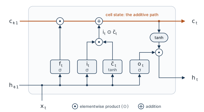
The trouble in Equation 7 is that every step forces the state through a multiplication by W and a \tanh. The long short-term memory network (LSTM; Hochreiter and Schmidhuber, 1997) adds a second state vector, the cell state c_t \in \mathbb{R}^{d_h}, which is updated additively, and gates that decide what to keep, write and reveal. A gate is a vector with entries in (0, 1), produced by a sigmoid, that multiplies another vector elementwise: 0 blocks, 1 passes.

One LSTM step takes x_t, h_{t-1} and c_{t-1} and computes:

\begin{aligned} f_t &= \sigma(W_f h_{t-1} + U_f x_t + b_f) && \text{forget gate: what to keep of } c_{t-1} \\ i_t &= \sigma(W_i h_{t-1} + U_i x_t + b_i) && \text{input gate: what to write} \\ o_t &= \sigma(W_o^{\text{g}} h_{t-1} + U_o x_t + b_o^{\text{g}}) && \text{output gate: what to reveal} \\ \tilde{c}_t &= \tanh(W_c h_{t-1} + U_c x_t + b_c) && \text{candidate values to write} \\ c_t &= f_t \odot c_{t-1} + i_t \odot \tilde{c}_t && \text{cell update} \\ h_t &= o_t \odot \tanh(c_t) && \text{hidden state} \end{aligned} \tag{10}

Symbols: f_t, i_t, o_t \in (0,1)^{d_h} are the three gates; \tilde{c}_t \in (-1,1)^{d_h} is the candidate; each gate and the candidate has its own recurrent matrix (W_f, W_i, W_o^{\text{g}}, W_c), input matrix (U_f, U_i, U_o, U_c) and bias. The superscript \text{g} on the output gate’s W_o^{\text{g}} and b_o^{\text{g}} only distinguishes them from the output layer’s W_o and b_o in Equation 2. The first four lines have the same form as Equation 1; an LSTM has four times the parameters of an RNN with the same d and d_h. The output layer Equation 2 and the loss Equation 3 are unchanged.

An LSTM cell: the cell state runs along the top, scaled by the forget gate and added to by the input gate; the output gate controls the hidden state. — Figure 2: One LSTM cell. The cell state runs along the top from c_{t-1} to c_t: it is multiplied elementwise by the forget gate f_t, then i_t \odot \tilde{c}_t is added. The output gate o_t scales \tanh(c_t) to give h_t.

def lstm_cell_step(x_t, h_prev, c_prev, p):
    # p holds W_*, U_*, b_* for f, i, o, c.  All states: (B, d_h)
    f = torch.sigmoid(h_prev @ p.W_f.T + x_t @ p.U_f.T + p.b_f)
    i = torch.sigmoid(h_prev @ p.W_i.T + x_t @ p.U_i.T + p.b_i)
    o = torch.sigmoid(h_prev @ p.W_o.T + x_t @ p.U_o.T + p.b_o)
    c_tilde = torch.tanh(h_prev @ p.W_c.T + x_t @ p.U_c.T + p.b_c)
    c = f * c_prev + i * c_tilde          # cell update
    h = o * torch.tanh(c)                 # hidden state
    return h, c

In the lab: Exercise 4 gives you the four gate lines and asks you to write the last two, the cell update and the hidden state of Equation 10. The checkpoint compares your step with nn.LSTMCell. After that the lab uses nn.LSTM, which is the same computation in optimized form.

Why This Helps the Gradient

Look at the cell update and differentiate c_t with respect to c_{t-1} along the direct path, holding the gates and the candidate fixed:

\frac{\partial c_t}{\partial c_{t-1}} = \mathrm{diag}(f_t) \quad \text{(direct path)}, \qquad \text{so} \qquad \frac{\partial c_t}{\partial c_s} = \prod_{j=s+1}^{t} \mathrm{diag}(f_j) \quad \text{(direct path)}. \tag{11}

Compare with Equation 7. There is no repeated matrix W and no \tanh' on this path, only the forget gates. Where the network sets an entry of f_j close to 1 over a span, the corresponding entry of the cell state, and the gradient with respect to it, pass through that span almost unchanged. Where it sets the entry close to 0, the memory is erased and so is the gradient, which is the correct behavior: nothing stored there should influence what follows.

Three honest qualifications.

The full Jacobian has further terms, because the gates and the candidate at step j depend on h_{j-1}, which depends on c_{j-1}. Equation 11 is the path that does not decay by construction, not the whole derivative.
The LSTM does not guarantee long memory. It makes long memory learnable: the forget gates are computed from the data, and the product in Equation 11 still shrinks whenever they are below 1.
LSTMs can still have exploding gradients, so clipping (Equation 9) stays on.

A practical detail that follows directly from Equation 11: implementations often initialize the forget-gate bias b_f to a positive value so that f_t starts close to 1 and gradients flow before the network has learned what to forget. The lab sets b_f = 1, so f_t \approx \sigma(1) \approx 0.73 at initialization instead of \sigma(0) = 0.5.

In the lab: after training, the gradient–distance measurement of Exercise 3 is repeated for the LSTM on the same 64 validation chunks, unrolled with your lstm_cell_step. The cell also prints the share of gate entries above 0.9 and 0.99, the units on which the direct path of Equation 11 barely decays. What the build run measured is in the box after the lab.

After the Lab: What Lab 3 Measured for the LSTM’s Gradient

Open this after the LSTM’s gradient plot, so that it does not answer the lab’s prediction for you. In the build run, 50 characters back the LSTM’s gradient was about 5 \times 10^{4} times the RNN’s. Its curve still falls: the trained forget gates average 0.74 over those chunks, well below 1.

Check yourself. At initialization the lab’s forget gates are about 0.73 on every unit. Along the direct path of Equation 11, what fraction of the gradient survives 50 steps? What constant gate value would let half of it survive 50 steps? And what does a unit with f_t = 1 and i_t = 0 do to its cell state?

Answer

0.73^{50} \approx 1.5 \times 10^{-7}: at initialization the direct path still decays fast, only more slowly than with f = 0.5. For half to survive, f^{50} = 0.5, so f = 0.5^{1/50} \approx 0.986. Long memory needs gates very close to 1, which is why the lab prints the share of gate entries above 0.99 and not just their mean. A unit with f_t = 1 and i_t = 0 computes c_t = c_{t-1}: it copies its cell state unchanged, and the gradient with it. The LSTM does not have long memory by default; it has a setting of the gates that gives long memory, and it can learn to use that setting on the units where it helps.

Optional: A Historical Note on the Forget Gate

The 1997 LSTM had no forget gate: the cell update was c_t = c_{t-1} + i_t \odot \tilde{c}_t, the “constant error carousel”, whose direct-path Jacobian is exactly the identity. The forget gate was added by Gers, Schmidhuber and Cummins (2000) so that the cell can reset itself on continual input streams. What is called “the LSTM” today, and what nn.LSTM implements, is the version with the forget gate.

The GRU in Brief

The gated recurrent unit (GRU; Cho et al., 2014) keeps the same idea, a gated additive update, with one state vector and two gates instead of two states and three gates. It has three quarters of the LSTM’s parameters and usually performs comparably. PyTorch provides it as nn.GRU, with the same interface as nn.LSTM minus the cell state. The lab uses the LSTM.

Optional: The GRU Equations

With an update gate u_t and a reset gate r_t, both in (0,1)^{d_h} (we write u_t where the literature writes z_t, because z is reserved for logits in this workshop):

\begin{aligned} u_t &= \sigma(W_u h_{t-1} + U_u x_t + b_u) \\ r_t &= \sigma(W_r h_{t-1} + U_r x_t + b_r) \\ \tilde{h}_t &= \tanh\big(W_h (r_t \odot h_{t-1}) + U_h x_t + b_h\big) \\ h_t &= u_t \odot h_{t-1} + (1 - u_t) \odot \tilde{h}_t \end{aligned}

The last line is the counterpart of the LSTM cell update: where u_t \approx 1 the state is copied forward and the direct-path Jacobian is close to the identity. This is the form in Cho et al. (2014). PyTorch’s nn.GRU applies the reset gate after the matrix product instead of before it; the difference does not change the idea.

6. Measuring the Improvement Fairly

In this section: compare perplexity against the n-gram baseline, and know when such a comparison means something.

Perplexity (Equation 4) is a per-token quantity, so its value depends on what a token is. A character-level model chooses among fewer than 100 symbols at each step; a word-level model chooses among tens of thousands. Their perplexities are on different scales and must not be compared. A character-level perplexity of 5 and a word-level perplexity of 150 say nothing about which model is better.

The lab’s language model is character-level. For the comparison with Module 1 to be valid, all of the following must hold, and the lab enforces each:

Same token unit. The baseline is the character n-gram model that Lab 1 already measured: counts c(\cdot) with add-k smoothing. Lab 3 restates Lab 1’s code and asserts that it reproduces Lab 1’s test values to four decimals. Lab 1’s word-level perplexities are never compared with these numbers.
Same data. The Tiny Shakespeare corpus from Lab 1, checked by hash, with the same fixed split by character position: 1,000,000 characters of train, 55,000 of validation, 60,394 of test.
Same vocabulary. All models assign probability over the same 65 characters of train.
Same scored positions. Every one of the 60,394 test characters is scored exactly once, by every model, and its left context is the true text before it, which for the first characters of the split is the end of the preceding split.
Same formula. Equation 4 with the natural logarithm, computed by the same function, your lm_loss_and_ppl.
No tuning on the test split. The smoothing constant k of each n-gram (from Lab 1’s grid) and the settings of the neural models are chosen on the validation split.

Character-level results are also often reported in bits per character, \mathrm{BPC} = \log_2 \mathrm{PPL} = \mathcal{L} / \ln 2, where \mathcal{L} is the mean loss in nats. It is the same measurement on a logarithmic scale; the lab prints both.

In the lab: the character n-gram baseline is provided as scaffolding, and your lm_loss_and_ppl from Exercise 2 scores it, the RNN and the LSTM. The results table is the checkpoint for the module’s third objective.

The two neural models are not trained at equal compute. The RNN (d_h = 256) trains for 1,000 steps and has 103,041 parameters; the LSTM (d_h = 256) trains for 2,000 steps (each step is 64 chunks of 128 characters) and has 350,593, about 3.4 times as many. So the table can show whether each recurrent model beats the counts, but not how much of any gap between the RNN and the LSTM is due to gating. The evidence for gating is the gradient measurement of Exercise 3 and its LSTM follow-up. The measured table is in the box after the lab, below.

After the Lab: What Lab 3 Measured

Open this after the lab’s results table, so that it does not answer the lab’s predictions for you. The checkpoint asserts that the LSTM’s test perplexity is at least 1.0 below the trigram’s and below the 5-gram’s.

These are the values measured by Lab 1 and Lab 3 and recorded in data/baselines.json (Lab 3 at full settings, seed 0, on a CPU, not yet on a Colab T4). All rows are on the same 60,394 test characters, in the same units.

Model	Lab	Test nats per character	Perplexity	Bits per character
Uniform over the 65 characters	–	4.1744	65	6.02
Character bigram, add-k (k = 0.1)	1	2.4922	12.09	3.60
Character trigram, add-k (k = 0.1)	1	2.0859	8.05	3.01
Best character n-gram, n \le 5: n = 5, add-k (k = 0.01)	1	1.8326	6.25	2.64
RNN, d_h = 256, 1,000 training steps (103,041 parameters)	3	1.6959	5.45	2.45
LSTM, d_h = 256, 2,000 training steps (350,593 parameters)	3	1.6114	5.01	2.32

Both neural models beat Lab 1’s best n-gram: the LSTM by 0.22 nats per character (perplexity 6.25 to 5.01), the RNN by 0.14. The RNN and LSTM rows are not at equal compute: the LSTM trained for twice as many steps (each step is 64 chunks of 128 characters) and has about 3.4 times the parameters. So the table shows that both recurrent models beat the counts; it does not isolate how much of the RNN–LSTM gap is due to gating. The evidence for gating is the gradient measurement of Exercise 3 and its LSTM follow-up.

Against the check below, with the numbers: the character LSTM’s 5.01 and Lab 1’s word trigram’s 1,437 are on different scales and say nothing about each other; the LSTM beats the character 5-gram, 5.01 against 6.25, on the same 60,394 test characters; and the LSTM’s 0.44 lead over the RNN (5.01 against 5.45) mixes gating with budget.

Check yourself. Before you see the lab’s numbers, decide what each of these perplexity comparisons can conclude. (a) The character LSTM against Lab 1’s word trigram, to say which model is better. (b) The LSTM against Lab 1’s character 5-gram on the same 60,394 test characters, scored by the same function, to say which predicts this text better. (c) The LSTM against the RNN, to say how much gating is worth.

Answer

Only (b) can conclude what it sets out to. Comparison (a) sets a per-character quantity against a per-word one; the two scales have nothing in common, and condition 1 fails whatever the numbers turn out to be. Comparison (b) meets all six conditions: same unit, data, vocabulary, scored positions, formula, and no tuning on test, so the lower number names the better predictor of this text. Comparison (c) is valid between two trained systems, since the units and the test text match, but not between two architectures: the LSTM gets twice the training steps and about 3.4 times the parameters, so any gap mixes gating with budget. A fair comparison answers the question “which number is lower”; it takes a controlled one to answer “why”.

Optional: Converting Between Character and Word Perplexity

If two models both assign a probability to the same complete test string, their total log-probabilities are comparable even when their token units differ. Let the test text contain N_c characters (counting spaces) and N_w words. A character model with total negative log-likelihood \mathrm{NLL} has \mathrm{PPL}_{\text{char}} = \exp(\mathrm{NLL}/N_c), and its implied per-word perplexity is

\exp(\mathrm{NLL}/N_w) = \mathrm{PPL}_{\text{char}}^{\,N_c / N_w}.

For example, if a text averages 5.5 characters per word including the space, a character perplexity of 4.5 corresponds to 4.5^{5.5} \approx 3{,}900 per word. The reverse conversion is usually not valid: a word-level model with a closed vocabulary maps rare words to an unknown-word token and so does not assign probability to the full string. This is why the lab compares like with like instead of converting.

7. Generating Text: Sampling Strategies

Not taught in the room. Lab 3’s Exercise 5 restates temperature sampling, the one strategy it asks you to write; top-k and nucleus sampling are its stretch section.

A trained language model gives a distribution \hat{y}_t over the next token. To generate, pick a token from it, feed that token back in as the next input, and repeat. How we pick matters.

Greedy decoding takes \arg\max_w \hat{y}_t[w] at every step. It is deterministic and tends to produce repetitive, looping text.

Sampling with temperature. Divide the logits by a temperature \tau > 0 before the softmax, then sample:

\hat{y}_t^{(\tau)} = \mathrm{softmax}(z_t / \tau), \qquad w_{t+1} \sim \hat{y}_t^{(\tau)}. \tag{12}

At \tau = 1 this samples from the model’s own distribution. As \tau \to 0 the largest logit dominates and sampling approaches greedy decoding. As \tau \to \infty the distribution approaches uniform. Temperature changes the sharpness of the distribution, never the ranking of tokens.

Worked example: one set of logits at three temperatures. Take a three-token vocabulary and logits z_t = (2, 1, 0). Equation 12 gives:

Temperature \tau	z_t / \tau	\hat{y}_t^{(\tau)}
0.5	(4, 2, 0)	(0.867,\ 0.117,\ 0.016)
1	(2, 1, 0)	(0.665,\ 0.245,\ 0.090)
2	(1, 0.5, 0)	(0.506,\ 0.307,\ 0.186)

Halving the temperature doubles every gap between logits, and the top token’s share rises from 0.665 to 0.867. Doubling it halves the gaps and the distribution moves toward uniform (0.333, 0.333, 0.333). In every row the order of the three tokens is the same.

Top-k sampling keeps the k most probable tokens, sets the rest to zero, renormalizes and samples. It removes the long tail of unlikely tokens, but k is fixed whether the model is confident or unsure.

Nucleus (top-p) sampling (Holtzman et al., 2020) keeps the smallest set of most probable tokens whose total probability is at least p, renormalizes and samples. The set is small when the model is confident and large when it is not.

def sample_with_temperature(logits, tau, generator=None):
    # logits: (..., |V|), one row per position z_t; returns one token ID per row, shape (...)
    probs = torch.softmax(logits / tau, dim=-1)                  # softmax(z_t / tau)
    flat = probs.reshape(-1, probs.shape[-1])                    # (N, |V|): multinomial wants 1-D or 2-D
    draws = torch.multinomial(flat, num_samples=1, generator=generator)  # (N, 1)
    return draws.reshape(probs.shape[:-1])

The explicit torch.Generator makes the draws reproducible from a seed.

In the lab: Exercise 5 asks you to write sample_with_temperature(logits, tau, generator), which is Equation 12. The checkpoint draws 20,000 samples at \tau \in \{0.5, 1, 2\} and checks the frequencies against \mathrm{softmax}(z/\tau), and checks that \tau = 0.01 always returns the arg max. You then generate 300 characters from the LSTM greedily and at \tau = 0.5, 1.0 and 1.5. Top-k and nucleus sampling are the stretch section (top_k_filter and nucleus_filter), whose filtered logits feed the same sampler. The same four strategies are how you will control generation from large models in Modules 7 and 8.

Check yourself. At one step the model’s distribution over four tokens is (0.50, 0.30, 0.15, 0.05). What does top-k sampling with k = 2 sample from? Nucleus sampling with p = 0.9? At the next step the model is confident: (0.95, 0.03, 0.01, 0.01). How many tokens does each method keep now?

Answer

First step. Top-2 keeps (0.50, 0.30) and renormalizes to (0.625, 0.375). Nucleus needs the smallest set with total at least 0.9: two tokens reach only 0.80, three reach 0.95, so it keeps three and renormalizes to (0.526, 0.316, 0.158). Second step. Top-2 still keeps two tokens, so it gives the 0.03 token a chance the model barely supports. Nucleus keeps one, because 0.95 already exceeds p, and the step is greedy. That is the difference in one example: k is the same at every step, while the size of the nucleus follows the model’s confidence.

Summary

An RNN applies one function at every position and carries a hidden state, so it conditions on the whole prefix instead of a fixed window (Equation 1, Equation 2).
It is trained with teacher forcing and cross-entropy; perplexity is the exponential of the mean loss (Equation 3, Equation 4).
The gradient linking distant positions is a product of Jacobians, each containing the same W. It shrinks or grows exponentially with distance (Equation 6, Equation 8). \lVert W \rVert < 1 guarantees vanishing, but it is not needed: the one-step Jacobians, whose \mathrm{diag}(1 - h_j^2) factors are near 0 for saturated units, can shrink the gradient even when \lVert W \rVert > 1. Lab 3 measures which case its trained RNN is in (the box after the lab in section 4).
Gradient clipping bounds the update and handles explosion (Equation 9). It does not address vanishing.
The LSTM adds a cell state with an additive, gated update. Along that path the Jacobian is a product of forget gates, which the network can hold near 1 (Equation 10, Equation 11). The GRU is a lighter variant of the same idea.
Perplexities are comparable only at the same token unit, on the same data, vocabulary and scored positions. Lab 3 compares the RNN and the LSTM with Lab 1’s character n-grams on those terms (the box after the lab in section 6).
Greedy, temperature, top-k and nucleus sampling trade off repetition against incoherence (Equation 12).

Equations and Where You Implement Them

Equation	What it is	In Lab 3
Equation 1	RNN step	Exercise 1: `rnn_cell_step`; Checkpoint 1 compares it with `nn.RNNCell`
Equation 2	Output layer and next-token distribution	Provided: `self.out` in `RNNLM` and `LSTMLM`
Equation 3, Equation 4, and BPC	Loss, perplexity, bits per character	Exercise 2: `lm_loss_and_ppl`; Checkpoint 2 tests the equal-logits case and agreement with `F.cross_entropy`
Equation 5, Equation 7	BPTT and the one-step Jacobian	Provided: autograd computes them in `train_lm` (`loss.backward()`)
Equation 6	Product of Jacobians	Exercise 3, part A: provided `grad_norm_by_distance` measures \lVert \partial \mathcal{L}_T / \partial h_s \rVert against the distance T - s; you predict the curve, then explain the measured one; Checkpoint 3A checks it
Equation 8	Bound by \lVert W \rVert^{t-s}	Exercise 3, part A: the printed `spectral_W`, \lVert W \rVert of the trained RNN; you compare it with 1 to decide what the bound alone can explain about the curve
Equation 9	Clipping by norm	Exercise 3, part B: `clip_gradients`; the provided `sgd_run` demonstration with and without it
Equation 10	LSTM step	Exercise 4: the last two lines of `lstm_cell_step`; Checkpoint 4 compares it with `nn.LSTMCell`
Equation 11	Direct-path Jacobian through the cell state	Provided: `grad_norm_by_distance` repeated for the LSTM, and the printed forget-gate statistics; you predict where the LSTM’s curve lies against the RNN’s, and a checkpoint compares the two at distance 50
Equation 12	Temperature sampling	Exercise 5: `sample_with_temperature`
Top-k and nucleus sampling	Tail filters	Stretch: `top_k_filter` and `nucleus_filter`
GRU (optional) and the character-to-word conversion (optional)	–	Not in the lab

Gotchas and Troubleshooting

“An RNN can use unlimited context.” In principle h_t depends on the whole prefix. In practice the usable context is limited by vanishing gradients, by the truncation length used in training, and by the fixed size of h_t.
“If \lVert W \rVert > 1, the gradient explodes.” \lVert W \rVert > 1 only removes the guarantee of vanishing. Saturated \tanh units pass almost no gradient back, so the gradient can vanish all the same (the worked example and the demo in section 4).
“Gradient clipping fixes vanishing gradients.” It only caps the size of the update. Vanishing is addressed by the architecture.
“The LSTM solves vanishing gradients.” It provides a path on which the gradient need not decay. Whether it decays depends on the learned forget gates, and LSTMs still struggle over many hundreds of steps.
“Vanishing gradients means the whole gradient is small.” The total gradient can be a healthy size. What vanishes is the contribution of distant positions relative to nearby ones.
“A lower perplexity always means a better model.” Only with the same token unit, the same test text and the same vocabulary. Character-level and word-level perplexities are different scales.
“Temperature changes what the model knows.” It reshapes one distribution at sampling time. The model, its ranking of tokens and its perplexity are unchanged.
“Teacher forcing is cheating.” It is ordinary maximum-likelihood training. Its cost is the train/generate mismatch (exposure bias), not an inflated score: held-out perplexity is also computed with the true prefix.

Next Steps

An RNN language model emits one output per input, in step with it. Many tasks instead map one sequence to another sequence of a different length: a sentence to its translation, “March 5, 2024” to “2024-03-05”. The natural move is to read the input with one RNN and take its final hidden state h_T as a summary from which a second RNN generates the output. That single fixed-size vector must then hold everything about the input, however long it is. Module 4 builds this encoder-decoder model, shows where the summary fails, and introduces attention to fix it.