The Transformer

Day 2 · Transformers and Pretraining Module 5 120 minutes (55 briefing, 55 lab, 10 debrief) 09:15 briefing · 10:10 lab · 11:05 debrief

Self-attention, multi-head attention and positional encodings, assembled into a small GPT.

Open the lab in Colab PyTorch

Duration: 120 minutes (55 briefing, 55 lab, 10 debrief)
Level: 300 · Advanced
Lab runtime: Google Colab, free T4 GPU · about 10 minutes of compute
Accounts and cost: Google. Free
Without API keys: the lab always runs its real models

What You Will Build

In this module you will:

Implement scaled dot-product attention with a causal mask
Inspect how heads, blocks and positions assemble into a decoder-only transformer
Train a small GPT with the provided loop and evaluate it against the LSTM

New terms, in the glossary: self-attention, causal mask, positional encoding, transformer block.

Before You Start

Module 4 · Seq2seq and Attention and its lab, and the modules before it: this module measures its results against theirs.
A Google account, and the Colab runtime set to T4 GPU (Runtime → Change runtime type).
No API keys: the lab runs its own models throughout.

Where we are. Day 1 ended with attention connecting any two positions in a single step, but attached to two recurrent networks that still read tokens one after another and still pass gradients along long chains. This module asks one question: if a sequence attends to itself and the recurrence is removed, what has to be added back (a mask, a sense of order, depth) to get a language model that trains in parallel?

In the Lab

Open the lab in Colab

6 exercises in 2 parts. The notebook budgets 50 minutes for them; the lab slot is 55 minutes. Each exercise you write is a # TODO stub with a folded solution beneath it and a checkpoint that passes or fails; where people tend to stall, a folded hint sits above the stub.

Task	Briefing section	Time
Part A · Building the Model
Exercise 0 · Read the Model	6, 7	3 min
Exercise 1 · Scaled Dot-Product Attention	2	12 min
Exercise 2 · The Causal Mask	3	8 min
Exercise 3 · Positions	5	6 min
Part B · Training and Comparing
Exercise 4 · Train the Mini-GPT and Compare It With the LSTM	7, 8	14 min
Exercise 5 · Looking at the Heads	4	7 min

Challenge · Write the Multi-Head Layer and the Block Yourself

Optional, for anyone who finishes the core path early: the notebook’s stretch section, after the last checkpoint.

When you are done. Runtime → Disconnect and delete runtime releases the machine; your keys stay in Colab Secrets for the next lab.

Agenda

Minutes	Section	In the room
0–5	1. From Attention Over an Encoder to Self-Attention	—
5–20	2. Scaled Dot-Product Attention	Demo (4 min); Check yourself (2 min)
20–27	3. The Causal Mask	Check yourself (2 min)
27–33	4. Multi-Head Attention	—
33–38	5. Positional Encodings	—
38–47	6. The Transformer Block	Check yourself (2 min)
47–51	7. A Decoder-Only Language Model, and the Other Two Variants	—
51–55	8. Cost and Parallelism	—
55	Total	45 minutes of exposition, 10 of activities

Checks, demos and predictions listed here are part of the live session and its minutes; the others on the page are for reading afterwards.

Read now · Sections 1–8, in the agenda above.

Use in the lab · Exercise 0: sections 6 and 7; Exercise 1: section 2; Exercise 2: section 3; Exercise 3: section 5; Exercise 4: sections 7 and 8; Exercise 5: section 4.

Read later · The collapsed callouts marked Optional or After the Lab; Further Reading.

1. From Attention Over an Encoder to Self-Attention

In this section: state what Module 4 left open and write self-attention as the query-key-value lookup with all three roles taken from one sequence.

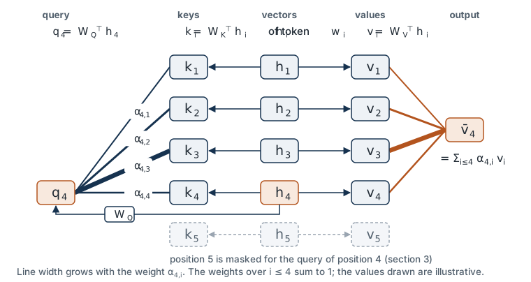
Module 4 ended with attention as a soft lookup. A query q is scored against keys k_1, \dots, k_S, a softmax turns the scores into weights \alpha_i, and the result is the weighted average of the values, \sum_i \alpha_i v_i. There the query was the decoder state, q = s_t, and the encoder states were both keys and values, k_i = v_i = h_i.

That model still had two recurrent networks, and Module 4 closed with two questions.

What if a sequence attends to itself? Take the queries, the keys and the values all from the same sequence. Then every position can read every other position in one step, with no encoder and decoder needed to set it up.
What if we then drop the recurrence? Recurrence is what made Modules 3 and 4 sequential (h_t waits for h_{t-1}) and what made distant positions hard to connect (the product of Jacobians in Module 3). If attention does the connecting, the recurrence may not be needed.

The transformer (Vaswani et al., 2017) answers yes to both. This module builds it for the task of Module 3: a language model over tokens w_1, \dots, w_T that predicts w_{t+1} from w_1, \dots, w_t.

Self-attention. Let h_1, \dots, h_T \in \mathbb{R}^d be the current vectors of the T positions of one sequence. (Where they come from is section 5; how layers stack is section 6.) The transformer uses a single width for embeddings and hidden vectors, so the hidden size d_h of Modules 3 and 4 equals the embedding dimension d here, and we write d throughout.

Each position plays all three roles, through three learned matrices:

q_t = W_Q^\top h_t, \qquad k_i = W_K^\top h_i, \qquad v_i = W_V^\top h_i , \tag{1}

with W_Q, W_K, W_V \in \mathbb{R}^{d \times d_k}. Here d_k is the dimension of the queries, keys and values. (Values may have their own dimension; we set it equal to d_k, as is usual.) The transposes appear because we are about to stack positions as rows of a matrix; see section 2.

Why three projections instead of using h_t directly, as Module 4’s dot-product score did? Because one vector now has three different jobs: what position t is looking for (q_t), what position i advertises (k_i), and what position i hands over when read (v_i). Module 4’s additive score already gave the query and the keys separate projections, W_q and W_k. The capital subscripts here mark that these are different matrices from those.

The rest is Module 4’s attention step, with position t asking and positions i answering:

\alpha_{t,i} = \frac{\exp\big(\mathrm{score}(q_t, k_i)\big)}{\sum_{j} \exp\big(\mathrm{score}(q_t, k_j)\big)}, \qquad \bar{v}_t = \sum_{i} \alpha_{t,i}\, v_i . \tag{2}

The output \bar{v}_t \in \mathbb{R}^{d_k} is a weighted average of values. The bar has the same meaning as in Module 4’s context vector \bar{h}_t, which was a weighted average of encoder states. There is one output per position, so a self-attention layer maps T vectors to T vectors.

Attention whose queries come from one sequence and whose keys and values come from another, as in Module 4, is called cross-attention. The table sets it beside self-attention. The first five rows are the lookup; the last four are what changes when the recurrence goes, and sections 3, 5 and 8 take them up.

General form	Module 4: cross-attention over a recurrent encoder	Self-attention, no recurrence
query q	decoder state s_t	W_Q^\top h_t, from position t
keys k_i	encoder states h_i	W_K^\top h_i, same sequence
values v_i	encoder states h_i	W_V^\top h_i, same sequence
weights	\alpha_{t,i}, target t on source i	\alpha_{t,i}, position t on position i
output	context vector \bar{h}_t	\bar{v}_t, one per position
what links the positions of one sequence	the recurrence: each state is computed from the one before	attention alone
steps that run one after another in training	one per token, in both networks	none within a layer: all T positions at once (section 8)
where word order comes from	the order of the recurrent steps	positional encodings added to the input (section 5)
typical failure	gradients fade along the recurrent chain (Module 3)	reading the future, unless a causal mask forbids it (section 3)

Self-attention for one position: its query is compared with the keys of the positions up to and including itself, and the output is the weighted average of their values. — Figure 1: Self-attention for one position. Position 4 asks: its query q_4 = W_Q^\top h_4 is scored against the keys k_1, \dots, k_4, and the output \bar{v}_4 = \sum_i \alpha_{4,i} v_i is the weighted average of the values. Line width grows with the weight \alpha_{4,i}; the weights drawn are illustrative. Position 5 is masked for this query (section 3).

Check yourself. To save parameters, someone ties the two projections: W_K = W_Q. With the dot-product score q_t^\top k_i, compare the score of position t reading position i with the score of position i reading position t. What kind of relation between two tokens can this layer no longer express?

Answer

The two scores are equal. With W_K = W_Q = W, the score is q_t^\top k_i = h_t^\top W W^\top h_i, and W W^\top is a symmetric matrix, so swapping t and i changes nothing. The layer can then express only mutual relevance. It cannot express a one-way relation, such as “a verb looks for its subject, but the subject is not looking for the verb”. The score of a position with itself, \lVert W^\top h_t \rVert^2, is also never negative, so each position tends to read itself. Separate matrices for the query and the key remove both limits: what a position asks for is no longer tied to what it advertises.

Check yourself. Apply the table to a new model. An image-captioning model has an encoder that turns a photo into 49 vectors, one per image patch, and a transformer decoder that writes the caption. Each decoder block has a causally masked self-attention layer and a cross-attention layer. (1) In each of the two layers, where do the queries, the keys and the values come from, and what shape is A when the caption so far has T tokens? (2) In training, what in the decoder has to run one position after another? And when a caption is generated? Sections 3, 7 and 8 give what you need.

Answer

In self-attention the queries, keys and values all come from the caption’s own vectors, and A is T \times T and lower triangular under the causal mask. In cross-attention the queries come from the decoder and the keys and values from the 49 patch vectors, so A is T \times 49, with no causal mask: the whole image is known. This is the encoder-decoder transformer of section 7’s optional box, with patches in place of source tokens. (2) In training, nothing within a layer: the whole caption is known (teacher forcing), so both layers compute all T positions at once, and the mask, not a recurrence, keeps each position from reading ahead. At generation the decoder runs once per token, because token t + 1 must be sampled before position t + 1 exists (section 8). The patch vectors do not depend on the caption, so the encoder runs once.

2. Scaled Dot-Product Attention

In this section: write the attention step in matrix form and derive the scaling factor 1/\sqrt{d_k}.

The score. Module 4 noted that multiplicative scores are cheap because they reduce to matrix products over all pairs at once. The transformer uses the dot product, divided by \sqrt{d_k}:

\mathrm{score}(q_t, k_i) = \frac{q_t^\top k_i}{\sqrt{d_k}} . \tag{3}

Matrix form. Stack the vectors as rows. H \in \mathbb{R}^{T \times d} has row t equal to h_t. Then

Q = H W_Q, \qquad K = H W_K, \qquad V = H W_V

are T \times d_k matrices whose rows are the q_t, k_i and v_i of Equation 1. The product Q K^\top is a T \times T matrix whose entry (t, i) is q_t^\top k_i: every score for the whole sequence in one matrix product. The whole step is

A = \mathrm{softmax}\!\left(\frac{Q K^\top}{\sqrt{d_k}}\right), \qquad \bar{V} = A\, V , \tag{4}

where the softmax is applied to each row separately. A \in \mathbb{R}^{T \times T} is the matrix of attention weights, with entry (t, i) equal to \alpha_{t,i} and each row summing to 1. It is the heat-map of Module 4, now square, with the same sequence on both axes. Row t of \bar{V} \in \mathbb{R}^{T \times d_k} is \bar{v}_t. This is Equation 2 for all positions at once.

In code, with any number of leading batch dimensions:

def scaled_dot_product_attention(Q, K, V, mask=None):
    # Q, K, V: (..., T, d_k)    mask: (T, T) bool, True where reading is allowed
    d_k = Q.size(-1)
    scores = Q @ K.transpose(-2, -1) / math.sqrt(d_k)       # (..., T, T)
    if mask is not None:
        scores = scores.masked_fill(~mask, float("-inf"))   # section 3
    A = torch.softmax(scores, dim=-1)                        # each row sums to 1
    V_bar = A @ V                                            # (..., T, d_k)
    return V_bar, A                                          # A: (..., T, T)

Why divide by \sqrt{d_k}. The argument is about variance, and it is the one given in a footnote of Vaswani et al. (2017). Write the dot product as a sum over the d_k coordinates, q^\top k = \sum_{j=1}^{d_k} q_j k_j, where q_j and k_j are the j-th coordinates of q and k. Assume, as is roughly true at initialization, that all coordinates are independent random variables with mean 0 and variance 1.

Each term has mean zero: \mathbb{E}[q_j k_j] = \mathbb{E}[q_j]\,\mathbb{E}[k_j] = 0, by independence.
Each term has variance one: \mathrm{Var}(q_j k_j) = \mathbb{E}[q_j^2 k_j^2] - 0^2 = \mathbb{E}[q_j^2]\,\mathbb{E}[k_j^2] = 1 \cdot 1 = 1.
The terms are independent, so their variances add: \mathrm{Var}(q^\top k) = d_k.

So the unscaled score has standard deviation \sqrt{d_k}: it grows with the dimension. Dividing a random variable by a constant divides its variance by the square of the constant, so

\mathrm{Var}\!\left(\frac{q^\top k}{\sqrt{d_k}}\right) = \frac{d_k}{d_k} = 1 \qquad \text{for every } d_k . \tag{5}

Why does the size of the scores matter? Because of the softmax. With d_k = 64 the unscaled scores have standard deviation 8. Two scores that differ by 8 get weights in the ratio e^{8} \approx 3000 to 1, so each row of A is close to one-hot from the first training step. And a one-hot softmax passes almost no gradient. Writing \mathrm{score}_j for \mathrm{score}(q_t, k_j), the derivative of the softmax is

\frac{\partial \alpha_{t,i}}{\partial\, \mathrm{score}_j} = \alpha_{t,i}\,\big(\mathbb{1}[i = j] - \alpha_{t,j}\big),

where \mathbb{1}[i=j] is 1 if i = j and 0 otherwise. Every entry is a product that contains either a weight near 0 or one minus a weight near 1, so every entry is near 0. The model would begin training with attention that is already saturated and hard to move. The scaling starts it with scores of unit size, whatever d_k is.

Note what the argument does and does not say. It is a statement about initialization. After training the coordinates are neither independent nor of unit variance, and the model can and does learn peaked attention where that is useful.

In the lab. Exercise 1 is scaled_dot_product_attention: Equation 3 and Equation 4. A provided cell then measures the standard deviation of the scores with and without the scaling for d_k = 16, 64, 256 on random unit-variance queries and keys, which is Equation 5 made visible; you predict the numbers first. Measured at seed 0: unscaled 4.006, 7.997 and 15.873 (against \sqrt{d_k} = 4, 8, 16); scaled 1.001, 1.000 and 0.992.

Worked example: one query and two keys, with and without the scaling. Take d_k = 4, a query q = (1, 1, 1, 1) and keys k_1 = (1, 1, 1, 1), k_2 = (1, -1, 1, -1). The dot products are q^\top k_1 = 4 and q^\top k_2 = 0.

	Scores	Weights (\alpha_1, \alpha_2)	\partial \alpha_1 / \partial\, \mathrm{score}_1 = \alpha_1 (1 - \alpha_1)
Without scaling	(4, 0)	(0.982,\ 0.018)	0.018
With 1/\sqrt{d_k} = 1/2 (Equation 3)	(2, 0)	(0.881,\ 0.119)	0.105

The scaling halves the gap between the scores. The row of weights is less extreme, and the derivative that carries the training signal back to the scores is about six times larger. At d_k = 4 the effect is mild. The gap between two typical unscaled scores grows as \sqrt{d_k}, so at d_k = 64 or 256 the unscaled row is close to one-hot for most random queries and keys, and its derivative is close to zero. The demo below shows this.

Try it: one row of attention at initialization. A query and the keys of ten positions are drawn at random, every coordinate independent with mean 0 and variance 1, as in the derivation above. The two panels show the same row of A computed from the same scores: on the left \mathrm{softmax}(q^\top k_i), on the right \mathrm{softmax}(q^\top k_i / \sqrt{d_k}) as in Equation 4.

Predict first. At d_k = 4 the two rows look similar. Raise d_k to 256. What happens to the largest weight in each row?

viewof dk = Inputs.select([4, 16, 64, 256, 1024], {value: 64, label: "Dimension dₖ"})
viewof draw = Inputs.range([1, 20], {value: 1, step: 1, label: "Random draw"})

{
  let state = 1000 * dk + draw;                          // seeded generator, so each setting is reproducible
  const uniform = () => {
    state = (state + 0x6D2B79F5) | 0;
    let t = Math.imul(state ^ (state >>> 15), 1 | state);
    t = (t + Math.imul(t ^ (t >>> 7), 61 | t)) ^ t;
    return ((t ^ (t >>> 14)) >>> 0) / 4294967296;
  };
  const normal = () => Math.sqrt(-2 * Math.log(1 - uniform())) * Math.cos(2 * Math.PI * uniform());
  const vector = () => Array.from({length: dk}, normal);
  const q = vector();
  const scores = Array.from({length: 200}, () => vector().reduce((s, kj, j) => s + q[j] * kj, 0));   // q^T k_i
  const softmax = (z) => {
    const top = Math.max(...z), e = z.map((v) => Math.exp(v - top)), total = e.reduce((a, b) => a + b, 0);
    return e.map((v) => v / total);
  };
  const sd = (z) => {
    const mean = z.reduce((a, b) => a + b, 0) / z.length;
    return Math.sqrt(z.reduce((a, b) => a + (b - mean) ** 2, 0) / z.length);
  };
  const row = scores.slice(0, 10), plain = "without scaling", scaled = "with 1/√dₖ";
  const a = softmax(row), b = softmax(row.map((s) => s / Math.sqrt(dk)));
  const rows = [...a.map((alpha, i) => ({i: i + 1, alpha, kind: plain})), ...b.map((alpha, i) => ({i: i + 1, alpha, kind: scaled}))];
  const chart = Plot.plot({
    width: 680, height: 280, marginBottom: 40,
    fx: {label: null, domain: [plain, scaled]}, x: {label: "position i"}, y: {label: "attention weight α", domain: [0, 1]},
    color: {domain: [plain, scaled], range: ["var(--demo-orange)", "var(--demo-blue)"]},
    marks: [Plot.barY(rows, {fx: "kind", x: "i", y: "alpha", fill: "kind"}), Plot.ruleY([0])]
  });
  return html`${chart}<p>Standard deviation of 200 scores for this query: ${sd(scores).toFixed(2)} without scaling (√dₖ = ${Math.sqrt(dk)}), ${(sd(scores) / Math.sqrt(dk)).toFixed(2)} with it.
  Largest of the ten weights: ${Math.max(...a).toFixed(3)} without scaling, ${Math.max(...b).toFixed(3)} with it.</p>`;
}

Without the scaling, the spread of the scores grows as \sqrt{d_k} (Equation 5), and the row collapses onto a single position as d_k grows: by d_k = 256 the largest weight is close to 1 on most draws. With the scaling the scores have a spread of about 1 at every d_k, and the row keeps the same moderate shape. The vectors here are random, so this is a picture of the first training step only. It says nothing about what a trained model’s attention looks like.

Check yourself. A colleague misremembers the formula and divides the scores by d_k instead of \sqrt{d_k}. Under the assumptions of the derivation, what is the standard deviation of the scores at d_k = 64? What does a row of A look like at initialization, and is that a problem?

Answer

Dividing by d_k divides the variance by d_k^2: \mathrm{Var} = d_k / d_k^2 = 1/d_k, so the standard deviation is 1/\sqrt{64} = 0.125. The scores are almost equal, so every row of A is almost uniform, and each \bar{v}_t is close to the plain average of the values it may read. This is the opposite failure from the unscaled one. The softmax is not saturated, so gradients do flow, but the layer starts out as an averaging machine that barely distinguishes one position from another, and the larger d_k is, the closer to uniform it starts. The exponent 1/2 is the only one for which the starting spread of the scores does not depend on d_k at all.

3. The Causal Mask

In this section: explain why a language model must not read ahead, and write the mask that prevents it.

As written, Equation 4 lets position t read every position, including those after it. For a language model that is fatal. The model is trained with teacher forcing (Module 3): one forward pass over w_1, \dots, w_T produces all T predictions, and the prediction at position t is scored against w_{t+1}. If position t can read position t+1, it can copy the answer. The training loss would fall toward zero, and the model would be useless at generation time, when the future does not exist yet.

An RNN could not make this mistake: h_t was computed before w_{t+1} was read. A transformer computes all positions at once, so the ordering has to be imposed.

We impose it exactly as Module 4 removed padded positions: set the forbidden scores to -\infty before the softmax, since \exp(-\infty) = 0. Define the causal mask M \in \mathbb{R}^{T \times T} by

M_{t,i} = \begin{cases} 0 & \text{if } i \le t, \\ -\infty & \text{if } i > t, \end{cases} \qquad A = \mathrm{softmax}\!\left(\frac{Q K^\top}{\sqrt{d_k}} + M\right). \tag{6}

M is zero on and below the diagonal and -\infty above it. Consequently \alpha_{t,i} = 0 exactly for i > t, each row of A still sums to 1 over the allowed positions i \le t, and A is lower triangular. Row t always has at least one allowed entry, the diagonal, so no row is empty.

mask = torch.tril(torch.ones(T, T, dtype=torch.bool))   # True where i <= t

With the mask in place, the output at position t is a function of w_1, \dots, w_t only, and one forward pass gives T valid next-token predictions, as in Module 3. This holds for the whole network only if no other component mixes positions; section 6 checks that.

The property is testable, and the test is the most useful one in the lab: change a token at position t_0, and the outputs at all positions before t_0 must not change at all.

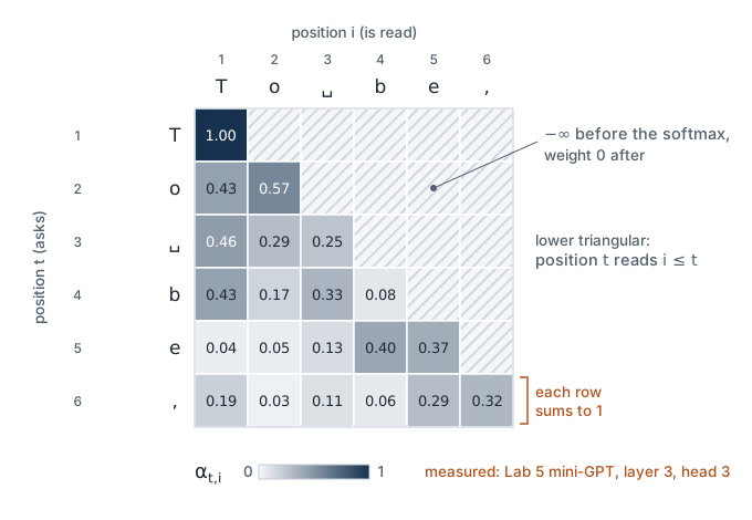
A lower-triangular six-by-six matrix of attention weights measured from one head of the Lab 5 model on the characters of To be: each position reads only itself and earlier positions, and the cells above the diagonal are hatched with weight zero. — Figure 2: The causal mask for the six characters of `To be,`. Row t holds the weights \alpha_{t,i} of position t. Cells above the diagonal have score -\infty before the softmax and weight 0 after it, so A is lower triangular and each row sums to 1 over i \le t (Equation 6). The weights are measured: layer 3, head 3 of the mini-GPT trained in Lab 5, reading these six characters. They are rounded to two decimals, so a printed row can sum to 0.99 or 1.01. The other 15 heads show other patterns; this one was chosen because it spreads its weight, which fills the triangle.

In the lab. In Exercise 2 you build the mask of Equation 6 and pass it to your attention function. The checkpoint is the leak test: weights above the diagonal are exactly zero, and changing a later token leaves all earlier outputs unchanged. The same test is then run on the logits of the whole model twice: on the untrained model at the end of Exercise 3, as soon as the model is complete, and on the trained model after training (Checkpoint 4b). Both run in evaluation mode, with dropout off. In the measured run the logits before the changed position moved by exactly 0.0 both times.

Check yourself. Row t = 2 of the scaled scores for a four-token sequence is (1, 1, 5, 3). What is row 2 of A under Equation 6? Now a buggy implementation applies the softmax to all four scores first and then sets the weights of positions 3 and 4 to zero, without renormalizing. What does it return, and does it leak the future?

Answer

Correct: the scores become (1, 1, -\infty, -\infty) and the row is (0.5, 0.5, 0, 0). Buggy: the softmax of (1, 1, 5, 3) is (0.016, 0.016, 0.853, 0.115), and zeroing the last two leaves (0.016, 0.016, 0, 0), a row that sums to 0.03. It does leak. The weights above the diagonal are zero, so a check of the triangle passes, but the surviving weights were divided by a sum that includes the future scores. Change the later tokens so that the scores are (1, 1, 0, 0) and the same code returns (0.366, 0.366, 0, 0): the output at position 2 moved when only the future changed. This is why the lab’s leak test changes a later token and compares earlier outputs, and does not stop at inspecting the triangle. (Renormalizing after zeroing gives (0.5, 0.5, 0, 0) again, which equals masking first.)

4. Multi-Head Attention

In this section: explain what one attention head cannot do, and write the multi-head layer and its split.

A softmax gives each position one distribution over the positions it reads, and one weighted average. But a position often needs several unrelated things at once. To predict the next character of a play, it helps to know the last few characters (to finish the word), and also who is speaking (to choose the vocabulary), which was settled far back. A single average of the two blurs them.

Multi-head attention runs n_h attention steps side by side. Each is called a head; head r has its own projections W_Q^{(r)}, W_K^{(r)}, W_V^{(r)} \in \mathbb{R}^{d \times d_k} and so its own weight matrix A^{(r)} and output \bar{V}^{(r)} = A^{(r)}\, H W_V^{(r)}, computed by Equation 4 with the mask of Equation 6. The outputs are concatenated along the columns and mixed by one more linear layer:

\mathrm{MHA}(H) = \big[\, \bar{V}^{(1)} ; \dots ; \bar{V}^{(n_h)} \big]\, W_{\mathrm{proj}} + b_{\mathrm{proj}} . \tag{7}

The head size is chosen as

d_k = \frac{d}{n_h},

so the concatenation has n_h d_k = d columns, W_{\mathrm{proj}} \in \mathbb{R}^{d \times d}, b_{\mathrm{proj}} \in \mathbb{R}^{d} (added to every row), and the layer maps T \times d to T \times d. We write W_{\mathrm{proj}} and not W_O, as the original paper does, because W_o is this workshop’s output layer.

The cost is the same as one big head. The n_h heads together hold 3 \cdot n_h \cdot d \cdot d_k = 3 d^2 projection weights, exactly what a single head with d_k = d would hold. Multi-head attention does not add capacity; it spends the same capacity on n_h separate, narrower lookups.

The split. In code nobody loops over heads. One d \times d matrix produces all the queries, and a reshape cuts the result into heads: columns (r-1) d_k + 1 to r\, d_k of that matrix are W_Q^{(r)}. The head index becomes a batch dimension, so the attention function of section 2 runs unchanged.

B, T, d = H.shape                                         # batch, positions, width
Q = self.W_Q(H).view(B, T, n_h, d_k).transpose(1, 2)      # (B, n_h, T, d_k)
K = self.W_K(H).view(B, T, n_h, d_k).transpose(1, 2)      # (B, n_h, T, d_k)
V = self.W_V(H).view(B, T, n_h, d_k).transpose(1, 2)      # (B, n_h, T, d_k)
V_bar, A = scaled_dot_product_attention(Q, K, V, mask)    # (B, n_h, T, d_k), (B, n_h, T, T)
V_bar = V_bar.transpose(1, 2).reshape(B, T, d)            # concatenate the heads
out = self.proj(V_bar)                                    # (B, T, d): W_proj, b_proj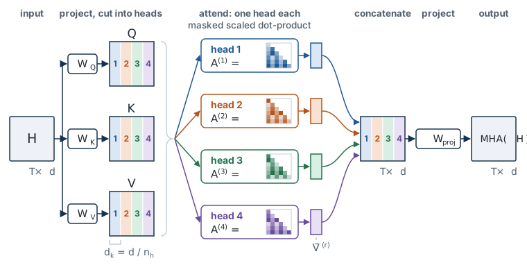

Multi-head attention: the projected queries, keys and values are cut into heads, each head attends separately, and the head outputs are concatenated and projected. — Figure 3: Multi-head attention with n_h = 4. Q, K and V are each cut into four slices of width d_k = d / n_h. Head r runs masked scaled dot-product attention on its slices and returns A^{(r)} and \bar{V}^{(r)}; the four outputs are concatenated and projected by W_{\mathrm{proj}} (Equation 7).

In the lab. The multi-head layer (Equation 7) is provided in the core path and calls your attention function with the head as a batch dimension, which is why Exercise 1 must accept leading dimensions. In Exercise 5 you summarize every head of the trained model by its mean attention distance (16 heads: 4 layers of 4) and plot A^{(r)} for every head of the first and the last layer. Writing the split yourself is the stretch section (MyMultiHeadAttention).

Check yourself. The lab’s model has d = 128 and n_h = 4. How many weights do W_Q, W_K and W_V hold across all heads of one layer? Change to n_h = 16 and count again. What did change, and what did you trade?

Answer

With n_h = 4: d_k = 128/4 = 32, and 3 \cdot n_h \cdot d \cdot d_k = 3 \times 4 \times 128 \times 32 = 49{,}152 = 3 d^2. With n_h = 16: d_k = 8, and 3 \times 16 \times 128 \times 8 = 49{,}152 again. The parameter count is the same. What changed is the shape of the computation: sixteen rows of weights per position instead of four, each from a score computed in an 8-dimensional space instead of a 32-dimensional one. You trade the precision of each lookup for the number of separate things a position can read at once. Push it to d_k = 1 and each head compares two numbers, which can say little about which position to read.

5. Positional Encodings

In this section: show that self-attention ignores order, and give two ways to restore it.

Look again at Equation 2. Position t’s output is a sum over the positions it reads, and each term depends only on the contents h_t and h_i. The index i appears nowhere except as a label on the sum. Shuffle the earlier positions and the same terms are added in a different order: \bar{v}_t is unchanged. A self-attention layer treats what it reads as a set, not a sequence. This is the blind spot of Module 2’s averaged embeddings again: “dog bites man” and “man bites dog”.

An RNN had order built into its computation. A transformer has to be told. The fix is to add to each token embedding a vector that depends only on the position. Writing h_t^{(0)} for the input to the first layer,

h_t^{(0)} = e_{w_t} + p_t , \tag{8}

where e_{w_t} \in \mathbb{R}^d is the embedding of token w_t (Module 2) and p_t \in \mathbb{R}^d is the positional encoding of position t. The same token at two positions now has two different vectors, so queries and keys can depend on position.

Learned. Treat p_1, \dots, p_{T_{\max}} as parameters: a second embedding table, indexed by position instead of by token, trained with everything else. T_{\max} is the context length, the longest sequence the model accepts. This is what GPT-style models and the lab use. Its limit is plain: there is no p_t for t > T_{\max}.

Sinusoidal (Vaswani et al., 2017). Fix p_t by formula, with no parameters. For coordinate pairs j = 0, \dots, d/2 - 1,

p_{t,\,2j} = \sin(\omega_j t), \qquad p_{t,\,2j+1} = \cos(\omega_j t), \qquad \omega_j = 10000^{-2j/d} . \tag{9}

Each pair of coordinates is a point moving around a circle at its own frequency \omega_j, fast for small j and slow for large j, like the hands of a clock with d/2 hands. Because of the angle-addition formulas, p_{t+\Delta} is a fixed rotation of p_t for any offset \Delta, which makes “\Delta positions back” a pattern a linear layer can pick up. Vaswani et al. report that learned and sinusoidal encodings performed nearly the same in their experiments.

Both are absolute encodings: they mark where a token is, and leave the model to work out how far apart two tokens are. Many current models encode the relative offset inside the attention score instead.

Optional: Rotary Position Embeddings (RoPE)

Rotary embeddings (Su et al., 2021) add nothing to the input. They act inside each attention layer, on the queries and keys only.

Group the d_k coordinates of a query into d_k/2 pairs and treat each pair as a point in the plane. Before taking the dot product, rotate pair j of q_t by the angle \omega_j t, and pair j of k_i by the angle \omega_j i, with frequencies \omega_j as in Equation 9 (with d_k in place of d). Write R_t for this block-wise rotation at position t. Rotations preserve length, and the dot product of two rotated vectors depends only on the difference of the angles:

(R_t\, q_t)^\top (R_i\, k_i) = q_t^\top R_{i-t}\, k_i .

So the score depends on the positions only through the offset i - t: the encoding is absolute in how it is applied (each vector is rotated by its own position) and relative in its effect. The values are not rotated. In the words of the paper’s abstract, RoPE “encodes the absolute position with a rotation matrix and meanwhile incorporates the explicit relative position dependency in self-attention formulation”.

Not covered in the lab.

In the lab. In Exercise 3 you write the input step of the model, Equation 8 with a learned position table: embed_with_positions(idx, tok_emb, pos_emb). Before you do, a checkpoint on a single attention layer shows the problem: with positions left out, shuffling the earlier tokens leaves the last position’s output unchanged. Sinusoidal encodings (Equation 9) are not implemented in the lab.

Check yourself. Leave out the positional encodings but keep the causal mask. Feed a single attention layer dog bites man and then bites dog man. Is the output at position 3 the same? Now stack a second attention layer on top. Is the output at position 3 still the same?

Answer

One layer: the same. In both orders position 3 holds man and reads the set {dog, bites, man}, and Equation 2 depends only on the contents. Two layers: in general, different. The first layer’s outputs at positions 1 and 2 are not the same in the two orders. In dog bites man, position 1 is dog having read only itself and position 2 is bites having read {dog, bites}. In bites dog man, position 1 is bites alone and position 2 is dog having read both. The second layer at position 3 reads these vectors, so it receives a different set. The causal mask therefore lets some order information in, because how much a position may read depends on where it is. That signal is weak and indirect, which is why the model is still given Equation 8.

6. The Transformer Block

In this section: assemble attention, a feed-forward layer, residual connections and layer normalization into one block, and say where the normalization goes.

Attention moves information between positions. It does little computation at a position: \bar{v}_t is a linear function of the values. The block therefore pairs attention with an ordinary feed-forward network, and adds two devices that make a deep stack trainable.

Feed-forward layer. A network with one hidden layer, as in Module 2, applied to each position separately and with the same weights at every position:

\mathrm{FFN}(h) = W_2\, g(W_1 h + b_1) + b_2 , \tag{10}

with W_1 \in \mathbb{R}^{d_{\mathrm{ff}} \times d}, b_1 \in \mathbb{R}^{d_{\mathrm{ff}}}, W_2 \in \mathbb{R}^{d \times d_{\mathrm{ff}}}, b_2 \in \mathbb{R}^{d}. The hidden width d_{\mathrm{ff}} is usually 4d. The nonlinearity g is applied elementwise: ReLU, g(a) = \max(0, a), in the original paper; GPT models and the lab use GELU, a smooth variant.

Layer normalization (Ba et al., 2016). Rescale one vector h \in \mathbb{R}^d to zero mean and unit variance across its own d coordinates, then apply a learned gain and bias:

\mathrm{LN}(h) = \gamma \odot \frac{h - \mathrm{mean}(h)}{\sqrt{\mathrm{var}(h) + \epsilon}} + \beta , \tag{11}

where \mathrm{mean}(h) and \mathrm{var}(h) are the mean and variance of the d coordinates of h, \gamma, \beta \in \mathbb{R}^d are learned (initialized to ones and zeros), \odot is the elementwise product, and \epsilon is a small constant that prevents division by zero. It keeps the scale of the vectors steady from layer to layer. Note that it uses only the vector itself: not other examples in the batch, and not other positions.

Residual connections. Each sublayer adds its output to its input instead of replacing it. One block, layer \ell of n_\ell, with H^{(\ell-1)} \in \mathbb{R}^{T \times d} the matrix of vectors entering it, \mathrm{LN} and \mathrm{FFN} applied to each row, and H' the intermediate result:

\begin{aligned} H' &= H^{(\ell-1)} + \mathrm{MHA}\big(\mathrm{LN}(H^{(\ell-1)})\big), \\ H^{(\ell)} &= H' + \mathrm{FFN}\big(\mathrm{LN}(H')\big). \end{aligned} \tag{12}

Each block has its own parameters. Row t of H^{(\ell)} is h_t^{(\ell)}, the vector of position t after layer \ell.

Why add? For the reason the LSTM cell state was additive in Module 3. Unroll Equation 12 over the layers:

H^{(n_\ell)} = H^{(0)} + \sum (\text{outputs of all } 2 n_\ell \text{ sublayers}) .

The vectors run straight through the network, and each sublayer reads them and writes a correction. This running sum is often called the residual stream. The derivative of a block’s output with respect to its input is the identity matrix plus the derivative of the corrections, so the gradient reaches the first layer through a path with no repeated matrix product on it. Compare the product of Jacobians that made the RNN’s gradient vanish.

Pre-norm and post-norm. Equation 12 normalizes the input of each sublayer. This is the pre-norm arrangement, used by GPT-2, by most later models and by the lab. The original transformer normalized after the addition (post-norm):

H' = \mathrm{LN}\big(H^{(\ell-1)} + \mathrm{MHA}(H^{(\ell-1)})\big), \qquad H^{(\ell)} = \mathrm{LN}\big(H' + \mathrm{FFN}(H')\big). \tag{13}

The difference is what lies on the residual path. In post-norm every block passes the running sum through a normalization, so there is no untouched identity path from input to output. In pre-norm there is. Xiong et al. (2020) analyze the two at initialization: in post-norm the gradients of the parameters near the output are large, which is why the original recipe needs a careful learning-rate warm-up; in pre-norm the gradients are well-behaved and the warm-up can be removed. Two consequences to remember:

Pre-norm leaves the output of the last block unnormalized, so one final \mathrm{LN} is applied before the output layer (section 7).
This is a statement about ease of training, not a ranking. Post-norm models train well with a suitable schedule.

Does the block respect the causal mask? Yes. \mathrm{LN} and \mathrm{FFN} act on each position separately, and the residual additions are position by position. The masked attention is the only place where positions exchange information, so the argument of section 3 carries through any number of blocks. (Batch normalization, which mixes examples, would not be so harmless; this is one reason transformers use layer normalization.)

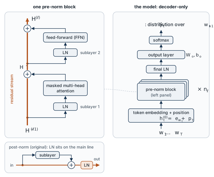
Figure 4: Left: one pre-norm block (Equation 12). The residual stream runs from H^{(\ell-1)} to H^{(\ell)}; each sublayer reads a normalized copy of it and adds its output back. Inset: in the original post-norm block (Equation 13) the normalization sits on the main line, after the addition. Right: the decoder-only model (Equation 14), with n_\ell blocks between the embeddings and the output layer.

In the lab. The block (Equation 12), with Equation 10 and Equation 11 inside it, is provided in the core path; you read it and find your attention function in it. Writing the full block yourself is the stretch section.

Check yourself. Let h = (1, 2, 3, 6), with \gamma all ones, \beta all zeros and \epsilon negligible. Compute \mathrm{LN}(h) from Equation 11. Without further arithmetic, what is \mathrm{LN}(10h + 5)? What does that mean for a sublayer in a pre-norm block when the residual stream grows from layer to layer?

Answer

The mean is 3 and the variance is (4 + 1 + 0 + 9)/4 = 3.5, with square root 1.871, so \mathrm{LN}(h) = (-1.07,\ -0.53,\ 0,\ 1.60). \mathrm{LN}(10h + 5) is the same vector: adding 5 to every coordinate is removed by subtracting the mean, and the factor 10 is removed by dividing by the standard deviation. Layer normalization keeps the pattern across coordinates and discards the overall scale and offset. In a pre-norm block each sublayer reads \mathrm{LN} of the residual stream, so its input has the same scale whether the stream has accumulated one correction or twenty. The stream itself is never rescaled along the way, which is why one final \mathrm{LN} is needed before the output layer.

7. A Decoder-Only Language Model, and the Other Two Variants

In this section: write the whole model from tokens to loss, and place it among the three transformer variants.

Everything is now in place. A decoder-only transformer, the architecture of the GPT models, is:

\begin{aligned} h_t^{(0)} &= e_{w_t} + p_t && \text{embed tokens and positions (section 5)} \\ H^{(\ell)} &= \mathrm{Block}_\ell\big(H^{(\ell-1)}\big), \quad \ell = 1, \dots, n_\ell && \text{blocks with causal masks (section 6)} \\ z_t &= W_o\, \mathrm{LN}\big(h_t^{(n_\ell)}\big) + b_o && \text{final normalization and output layer} \\ \hat{y}_t &= \mathrm{softmax}(z_t) && \text{distribution over } w_{t+1} \end{aligned} \tag{14}

with z_t \in \mathbb{R}^{|V|} the logits and W_o \in \mathbb{R}^{|V| \times d}, b_o \in \mathbb{R}^{|V|} the output layer, as in Module 3 with d in place of d_h. The parameters \theta are the two embedding tables, the blocks, the final normalization and the output layer.

Training is unchanged from Module 3: teacher forcing, the cross-entropy loss, and perplexity as its exponential, in nats:

\mathcal{L} = -\frac{1}{T}\sum_{t=1}^{T} \log \hat{y}_t[w_{t+1}], \qquad \mathrm{PPL} = \exp(\mathcal{L}). \tag{15}

Generation is also unchanged: sample w_{t+1} from \mathrm{softmax}(z_t/\tau) with temperature \tau, append it, and repeat. The one new constraint is the context length: once the text is longer than T_{\max}, the model sees only the last T_{\max} tokens. An LSTM carries its state forward indefinitely; a transformer has perfect access to everything inside its window and none to anything outside it.

The three variants. They differ in the mask and in what is attended to.

Variant	Mask	Each position reads	Example	In this workshop
Decoder-only	causal	itself and earlier positions	GPT	this lab; Modules 7 to 10
Encoder-only	none	all positions, both sides	BERT	Module 6
Encoder-decoder	none in the encoder, causal in the decoder	the decoder also reads the encoder’s output	the original transformer, T5	not built

An encoder cannot generate text left to right, because its vectors depend on tokens to the right. It produces a representation of a whole input, which suits classification. Module 6 takes this up.

Optional: The Encoder-Decoder Transformer and Cross-Attention

The original transformer was built for translation, the task of Module 4, and keeps Module 4’s two-part shape.

The encoder is a stack of blocks as in Equation 12 with no causal mask. Its output is one vector per source position: the counterpart of Module 4’s encoder states h_1, \dots, h_S.
The decoder is a stack of blocks with three sublayers each: causally masked self-attention over the target so far, then cross-attention, then the feed-forward layer. Each has its own residual connection and layer normalization.

Cross-attention is Equation 4 with the queries taken from the decoder and the keys and values taken from the encoder output. Let H_{\mathrm{dec}} hold the decoder’s current vectors and H_{\mathrm{enc}} the encoder’s final ones:

Q = H_{\mathrm{dec}} W_Q, \qquad K = H_{\mathrm{enc}} W_K, \qquad V = H_{\mathrm{enc}} W_V .

Here A is T \times S, not square, and there is no causal mask on it: the whole source is known. This is exactly Module 4’s attention: the query comes from the decoder, the keys and values from the encoder. What changed is the score (scaled dot product), the number of heads, and that it happens in every decoder block instead of once.

Padding is handled as in Module 4: the scores of padded source positions are set to -\infty, in the encoder’s self-attention and in cross-attention.

A decoder-only model handles a transduction task by writing source and target as one sequence, with the source as the prefix. Self-attention over the prefix then does the work of cross-attention. This is how the instruction-following models of Module 7 work.

Optional: Details That Implementations Add

Dropout. The lab applies it in two places: to the input vectors h_t^{(0)}, after the embeddings are added, and to each sublayer’s output (after W_{\mathrm{proj}} in attention, after W_2 in the feed-forward layer), before the residual addition. Many implementations, nanoGPT among them, also apply it to the attention weights A; the lab does not. Dropout is switched off at evaluation, and the leak test in the lab runs with it off.
Weight tying. The output matrix W_o and the token embedding table have the same shape, |V| \times d, and many models share one matrix for both. The lab keeps them separate.
Bias terms. Some implementations add biases to the projections of Equation 1; we omit them, and so does the lab.
Caching at generation time. Under the causal mask, the keys and values of earlier positions do not change when a token is appended, so implementations store them and compute only the new position’s query at each step. The lab’s sampler does not cache: it re-reads the last T_{\max} characters at every step, which is simpler and fast enough for 300 characters.

In the lab. The assembled model (Equation 14) and the training loop are provided. Before training, a checkpoint confirms that the untrained model predicts almost uniformly: measured loss 4.1909 nats against \ln 65 = 4.1744. In Exercise 4 you train it on the Shakespeare corpus of Lab 3 and score it with Lab 3’s loss and perplexity (Equation 15) on the same 60,394 test characters, beside the character n-gram baselines and two LSTM rows.

Check yourself. The lab’s model has d = 128, n_\ell = 4 and T_{\max} = 128, with learned positions. You double the context length to T_{\max} = 256. Which parameters of Equation 14 grow, and by how many? What happens to the cost of the attention step on a full-length sequence? And with T_{\max} = 128, which characters of a 300-character text can influence the prediction of character 301?

Answer

Only the position table grows: it needs a vector p_t \in \mathbb{R}^{128} for each of 128 new positions, 128 \times 128 = 16{,}384 parameters on top of 824,897. No block changes, because attention, the feed-forward layer and layer normalization have no parameter that depends on the sequence length. The computation is another matter: the attention step costs O(T^2 d) per layer (section 8), so a full window of 256 costs four times as much as one of 128, and stores four times as many attention weights. With T_{\max} = 128, the prediction of character 301 depends on characters 173 to 300 and on nothing earlier. Unlike the LSTM’s fading memory, the cutoff is exact.

After the Lab: What Lab 5 Measured

Open this after Exercise 4, so that it does not answer the lab’s prediction for you. These are the values recorded in data/baselines.json (Lab 5 at its full settings, seed 0, executed on a CPU; not yet run on a Colab T4). Every row scores the same 60,394 test characters with the same function, in nats per character.

Model	Lab	Parameters	Training steps (batch 64)	Test nats per character	Perplexity	Bits per character
Character trigram, add-k (k = 0.1)	1	–	counts	2.0859	8.05	3.01
Character 5-gram, add-k (k = 0.01)	1	–	counts	1.8326	6.25	2.64
LSTM, d_h = 256, Lab 3’s own run (Adam, constant learning rate)	3	350,593	2,000	1.6114	5.01	2.32
LSTM, same architecture, retrained in Lab 5 with the GPT’s loop and budget	5	350,593	3,000	1.5727	4.82	2.27
Mini-GPT, d = 128, n_h = 4, n_\ell = 4, T_{\max} = 128	5	824,897	3,000	1.5481	4.70	2.23

How to read it:

Both neural models beat the counts by a wide margin: the mini-GPT is 0.28 nats per character below Lab 1’s best n-gram, and the lab asserts that it is well below the trigram.
The two LSTM rows are the same architecture with different training. The row retrained in Lab 5 uses the GPT’s training loop (AdamW, warm-up, cosine decay, a learning rate chosen on validation), batch size and number of steps. It is the fair partner for the GPT. The change of training moved the LSTM by 0.04 nats. (One other difference: Lab 5 keeps PyTorch’s default initialization and does not set the forget-gate bias to 1 as Lab 3 does.)
GPT against the retrained LSTM is a tie at this budget, not a ranking. The GPT is ahead by 0.025 nats from a single seed. In the lab’s shortened QUICK mode, three seeds of each model spread over 0.02 to 0.03 nats, about the size of that gap. In QUICK mode (batch 16, 1,500 steps) the LSTM wins clearly: 1.56 to 1.58 nats against 1.77 to 1.79 for the GPT, three seeds each. One reading is that the smaller recurrent model learns faster from little training and the transformer catches up given more; two budgets and a single seed at the larger one do not establish that trend.
The budget is stated, not equal. The GPT has 2.4 times the parameters. On the CPU used for the measurement it took about 11 times as long to train (3,921 seconds against 348). Those are CPU times on a shared machine, not T4 times; the ratio on a GPU, where the transformer’s work parallelizes over positions (section 8), has not been measured.
Same characters, different context. The LSTM carries its state across the whole test split. The GPT reads at most T_{\max} = 128 characters, so it is scored with overlapping windows of 128 moved forward by 64, scoring only the second half of each: every character has between 65 and 128 characters of context. The comparison is of the models as they are used, not of the architectures in isolation.

8. Cost and Parallelism

In this section: compare the cost of a self-attention layer with a recurrent layer, and say what the transformer gains and what it pays.

Count the multiplications for one layer over a sequence of length T.

Self-attention. There are T^2 pairs of positions. Each score is a dot product in d_k dimensions, in each of n_h heads: T^2 \cdot n_h d_k = T^2 d. The weighted averages cost the same. So the attention step costs O(T^2 d).
Recurrent layer. There are T steps. Each multiplies the hidden state by a d_h \times d_h matrix: O(T d_h^2), or O(T d^2) at equal width.

	Self-attention layer	Recurrent layer
Computation per layer	O(T^2 d)	O(T d^2)
Sequential operations	O(1)	O(T)
Longest path between two positions	O(1)	O(T)

(These three rows are Table 1 of Vaswani et al., 2017.) Reading the table:

Computation. Self-attention is cheaper when T < d and more expensive when T > d. It is quadratic in the sequence length: doubling the context quadruples the cost. It also stores T^2 weights per head in every layer.
Sequential operations. This is the row that changed the field. An RNN needs T steps one after another, because h_t waits for h_{t-1}; no amount of hardware removes the wait. In a self-attention layer no position waits for another, so all T are computed at once as matrix products, which is what a GPU is good at.
Path length. Any two positions are connected by one attention step, so a gradient between them does not pass through a product of T Jacobians. Module 3’s vanishing-gradient problem along the sequence does not arise.

Two honest additions.

The projections and the feed-forward layer of a full block cost O(T d^2) as well, so a transformer block costs O(T^2 d + T d^2). The table compares only the parts that connect positions.
Parallelism applies to training, where the whole sequence is known. Generation is still one token at a time: w_{t+1} must be sampled before position t+1 can be processed.

What the transformer pays: a fixed context length, a quadratic cost in it, and the loss of the built-in sense of order, bought back with positional encodings. What it gains: parallel training and short paths. Those two together are what made training on very large corpora practical, which is the subject of Module 6.

None of this says that a small transformer beats a small LSTM on a small corpus in a few minutes of training. That is an empirical question, and the lab measures it; the answer is in the after-the-lab note at the end of section 7. The advantages above matter most at scale, and a one-megabyte corpus with a few thousand training steps is far from it.

In the lab. The results table of Exercise 4 prints the parameter count, the number of steps and the training time beside test perplexity for every model, so the comparison is at a stated budget. The notebook deliberately asserts nothing about GPT against LSTM.

Check yourself. For the lab’s sizes, T = 128 and d = 128, compare T^2 d with T d^2. Then keep d = 128 and lengthen the sequence to T = 1{,}024: what is the ratio now? Finally, the lab’s sampler generates 300 characters. How many forward passes does that take, and how much of the transformer’s parallelism does it use?

Answer

At T = d = 128 the two are equal: 128^3 = 2{,}097{,}152 multiplications each. The ratio T^2 d / (T d^2) is T/d, so at T = 1{,}024 self-attention costs 8 times the recurrent layer, and each further doubling of T doubles the ratio. Generation takes 300 forward passes, one per character, because character t + 1 must be sampled before position t + 1 exists. The passes cannot run at the same time. Within one pass the positions are still computed in parallel, but only the last position’s output is used. The parallelism that changed the field is a property of training, where all T targets are known in advance.

Summary

Self-attention is Module 4’s query-key-value lookup with all three taken from one sequence, through learned projections (Equation 1, Equation 2).
In matrix form it is two matrix products and a row-wise softmax (Equation 4). Scores are divided by \sqrt{d_k} so that their variance is 1 at initialization whatever the dimension, which keeps the softmax out of its saturated region (Equation 5).
A causal mask sets the scores of later positions to -\infty, so position t depends only on w_1, \dots, w_t and one forward pass gives T valid predictions (Equation 6).
Multi-head attention runs n_h narrower lookups in parallel, with d_k = d / n_h, at the parameter cost of one (Equation 7).
Self-attention ignores order. Positional encodings, learned or sinusoidal, are added to the token embeddings to restore it (Equation 8, Equation 9).
A block is attention plus a feed-forward layer, each wrapped in a residual connection with layer normalization (Equation 12). Pre-norm normalizes each sublayer’s input and keeps an identity path through the network; post-norm, the original, normalizes after the addition (Equation 13).
A decoder-only transformer is embeddings, n_\ell blocks, a final normalization and Module 3’s output layer, trained with Module 3’s loss (Equation 14, Equation 15).
Per layer, self-attention costs O(T^2 d) against the RNN’s O(T d^2), with O(1) sequential operations and path length against O(T).

Equations and Where You Implement Them

Equation	Lab 5
Scaled dot-product attention (Equation 3, Equation 4)	Exercise 1: `scaled_dot_product_attention`
The variance of the scores (Equation 5)	Exercise 1 follow-up: provided measurement, you predict and explain
Causal mask (Equation 6)	Exercise 2: `causal_mask`, and the leak test on one attention step; then `model_leak_test` on the whole model, untrained (end of Exercise 3) and trained (Checkpoint 4b)
Token plus position input (Equation 8)	Exercise 3: `embed_with_positions(idx, tok_emb, pos_emb)`
The model, loss and perplexity (Equation 14, Equation 15)	Exercise 4: train, then score on the test split beside the n-grams and the two LSTM rows (provided `train_lm`, `evaluate_gpt`, `evaluate_lstm`)
The weight matrices A^{(r)} per head	Exercise 5: `mean_attention_distance`, then plot the heads of the first and last layer
Multi-head split and the full block (Equation 7, Equation 12)	Stretch: `MyMultiHeadAttention`, `MyBlock` (provided in the core path as `MultiHeadAttention`, `Block`)
Projections, feed-forward layer, layer normalization (Equation 1, Equation 10, Equation 11)	provided
Sinusoidal encodings, post-norm (Equation 9, Equation 13)	not implemented

Gotchas and Troubleshooting

“The transformer is attention and nothing else.” Each block also has a feed-forward layer, which holds about two thirds of the block’s weights when d_{\mathrm{ff}} = 4d, plus residual connections and layer normalization. Without the residual connections a deep stack does not train.
“The scaling by \sqrt{d_k} is a detail.” Without it the standard deviation of the scores grows as \sqrt{d_k} and the softmax starts saturated. It is also not a temperature you tune: it is fixed by the dimension. The sampling temperature \tau is a different thing, applied to the logits at generation time.
“The causal mask is only needed at training time.” The model was trained with it, so it must be applied at generation too. Position t’s vector must be computed the same way whether or not later tokens are present.
“More heads means more parameters.” With d_k = d / n_h the count is the same for any n_h. More heads means more, narrower lookups.
“Self-attention knows the order of the tokens.” It does not. Order enters only through the positional encodings (and, in a decoder, weakly through the mask, since position t can tell how many positions it is allowed to read).
“Pre-norm and post-norm are the same thing drawn differently.” They put different operations on the residual path and behave differently at initialization. The original paper is post-norm; GPT-2 and most later models are pre-norm.
“Transformers are faster than RNNs.” They are more parallel. Per layer they cost O(T^2 d), which is more than an RNN for long sequences, and generation is still sequential.
“A transformer has unlimited context.” It reads at most T_{\max} tokens, and nothing before them.
“An attention map explains the prediction.” Module 4’s caution applies with more force: there are n_h \times n_\ell maps, and the vectors being read at layer \ell are already mixtures of many tokens.

Next Steps

We now have the architecture. The model in the lab is tiny, reads characters, and is trained from scratch on one megabyte of text. Module 6 changes each of those: tokens become subwords, the model is trained once on a very large corpus and then reused (pretraining), and the two masks of section 7 give two training objectives, causal language modeling for decoders and masked language modeling for encoders. From there on we load transformers from the Hugging Face libraries instead of writing them.