RLHF

Day 3 · Using and Aligning LLMs Module 10 120 minutes (55 briefing, 55 lab, 10 debrief) 14:45 briefing · 15:40 lab · 16:35 debrief

The full reinforcement-learning-from-human-feedback pipeline, DPO, and the ways it goes wrong.

Open the lab in Colab PyTorch Hugging Face

Duration

120 minutes (55 briefing, 55 lab, 10 debrief)

Level

400 · Expert

Lab runtime

Google Colab, free T4 GPU · about 7 minutes of compute

Accounts and cost

Google. Free

Without API keys

an open model runs in place of the commercial one

What You Will Build

In this module you will:

• Describe the three-stage RLHF pipeline
• Optimize a small LM against a reward model with a KL constraint
• Apply DPO and compare
• Name RLHF’s failure modes and observe one

New terms, in the glossary: KL penalty, direct preference optimization (DPO).

Before You Start

• Module 9 · Reinforcement and Preference Learning and its lab, and the modules before it: this module measures its results against theirs.
• A Google account, and the Colab runtime set to T4 GPU (Runtime → Change runtime type).
• API keys are optional. Without them an open model runs in place of the commercial one.

Where we are. Module 9 built two tools and kept them apart: a policy gradient that can optimize any reward, and a reward model learned from comparisons. It also warned that a reward model can be trusted only on text like its training data. This module answers one question: how do we optimize a language model against a learned reward without letting the optimizer exploit the reward’s errors?

In the Lab

Open the lab in Colab

5 exercises in 2 parts. The notebook budgets 50 minutes for them; the lab slot is 55 minutes. Each exercise you write is a # TODO stub with a folded solution beneath it and a checkpoint that passes or fails; where people tend to stall, a folded hint sits above the stub.

Task	Briefing section	Time
Step 0 · The Reward Model and the Gold Rule on the Reference’s Samples	—	3 min
Part A · The Pieces of the Objective
Exercise 1 · Log-Probabilities of a Response	3	8 min
Exercise 2 · The Per-Token Reward With a KL Penalty	4	8 min
Exercise 3 · Exact KL, Then RLHF With a KL Penalty	3, 4	11 min
Exercise 4 · Remove the Penalty: Reward Hacking	1, 7	8 min
Part B · DPO
Exercise 5 · The DPO Loss	6	12 min

Challenge · The Reward–Drift Trade-Off

Optional, for anyone who finishes the core path early: the notebook’s stretch section, after the last checkpoint.

When you are done. Runtime → Disconnect and delete runtime releases the machine; your keys stay in Colab Secrets for the next lab.

Agenda

Minutes	Section	In the room
0–3	1. What Module 9 Left Open	—
3–9	2. The InstructGPT Pipeline	—
9–19	3. The KL-Regularized Objective	Check yourself (2 min)
19–26	4. Optimizing It: A Per-Token Penalty and the Policy Gradient	—
26–40	6. DPO: From the Optimal Policy to a Classification Loss	Check yourself (2 min)
40–55	7. Failure Modes	Demo (4 min); Discuss (2 min)
55	Total	45 minutes of exposition, 10 of activities

Checks, demos and predictions listed here are part of the live session and its minutes; the others on the page are for reading afterwards.

Read now · Sections 1–4, 6 and 7, in the agenda above.

Use in the lab · Exercise 1: section 3; Exercise 2: section 4; Exercise 3: sections 3 and 4; Exercise 4: sections 1 and 7; Exercise 5: section 6.

Read later · Section 5, PPO in Outline (Reference); the collapsed callouts marked Optional; Further Reading.

Notation for This Module

The workshop notation applies: tokens w_1, \dots, w_T, vocabulary V, parameters \theta, loss \mathcal{L}, the sigmoid \sigma(a) = 1/(1 + e^{-a}), natural logarithms. From Module 9 we keep:

Symbol	Meaning
x	a prompt: the token sequence the model is given
y = (y_1, \dots, y_{\lvert y \rvert})	a response: the tokens the model generates after x, with \lvert y \rvert its length
s_t = (x, y_{<t})	the state at step t: the prompt and the response so far
\pi_\theta(y_t \mid s_t)	the policy: the language model with parameters \theta, read as a distribution over the next token
r_\phi(x, y)	the reward model, with parameters \phi: one number for a whole response
(x, y_w, y_l)	a preference triple: response y_w was preferred to y_l for prompt x
G_t, b_t	the return from step t onward, and a baseline subtracted from it

New in this module:

Symbol	Meaning
\pi_{\text{ref}}	the reference policy: a frozen copy of the model we start from
\beta > 0	the KL coefficient: how much drift from \pi_{\text{ref}} costs
\mathrm{KL}(p \,\Vert\, q)	the Kullback–Leibler divergence of p from q (section 3)
\mathcal{D}_x, \mathcal{D}_{\text{pref}}	the distribution of prompts, and the dataset of preference triples
\pi^*, Z(x)	the optimal policy of the KL-regularized objective, and its normalizer (section 6)
\hat{r}_\theta(x, y)	the implicit reward of a policy (section 6)

Notation. Four clashes, resolved for this module.

• x and y. In Module 1, x was an input vector and y a class label. From here on, x is a prompt and y a response, both token sequences.
• \beta is the KL coefficient, a single number we choose. It is not the shift vector of layer normalization in Module 5.
• r is a reward. It is not the LoRA rank of Module 7.
• \epsilon in section 5 is PPO’s clipping range, not the small constant in layer normalization.

The value function in section 5 is written v_\psi in lowercase, because V is already the vocabulary (Module 1) and the value matrix (Module 5).

1. What Module 9 Left Open

In this section: say why plugging a learned reward into the policy gradient is not enough.

Recall the two tools of Module 9 in one line each. The policy gradient (REINFORCE) raises the probability of sampled responses in proportion to how much better than the baseline they scored. The reward model r_\phi, trained on pairwise preferences with the Bradley–Terry model

P(y_w \succ y_l \mid x) = \sigma\big(r_\phi(x, y_w) - r_\phi(x, y_l)\big),

turns a finite set of human comparisons into a function that can score any response.

The obvious next step is to use one tool on the other: sample responses from the language model, score them with r_\phi, and follow the policy gradient. This works for a while and then fails, for a reason that is built into the setup.

• r_\phi is accurate only where it was trained. Its training pairs were responses written by one model, the one we started from. On text unlike those responses, its scores are extrapolation.
• The optimizer looks for high scores, wherever they are. The policy gradient moves the policy toward whatever r_\phi rates highly. If r_\phi overrates some odd kind of text, the policy will find it, because finding high-scoring text is exactly what it is trained to do.

This is Goodhart’s law in a training loop: a measure that becomes a target stops being a good measure. Optimizing a policy against a learned reward is called reward hacking when the policy improves its reward-model score while getting worse by the standard the reward model was meant to stand for. You will produce it in the lab.

This module covers four things:

1. the pipeline used in practice (section 2);
2. the objective that keeps the policy near where r_\phi can be trusted, and how to optimize it (sections 3 to 5);
3. DPO, which reaches the same objective without a reward model or a sampling loop (section 6);
4. what still goes wrong when all of this is done correctly (section 7).

2. The InstructGPT Pipeline

In this section: name the three stages of RLHF, what each one produces, and why each one is there.

Reinforcement learning from human feedback (RLHF) is the name for training a language model against a reward learned from human judgments. The recipe most systems follow was set out for summarization by Stiennon et al. (2020) and for general instructions by Ouyang et al. (2022), whose models are called InstructGPT. It has three stages.

1. Supervised fine-tuning (SFT). People write good responses to a set of prompts. The pretrained model is fine-tuned on them with the masked next-token loss of Module 7. The result is \pi_{\text{SFT}}.
2. Reward model. For a new set of prompts, \pi_{\text{SFT}} samples several responses. People rank them, and each ranking is split into pairs. A reward model r_\phi, usually the same kind of transformer with its output layer replaced by a single number, is trained on the pairs with the Bradley–Terry loss of Module 9.
3. Policy optimization. The policy \pi_\theta starts as a copy of \pi_{\text{SFT}}. On a third set of prompts it samples responses, r_\phi scores them, and an RL algorithm (PPO, section 5) updates \theta to raise the reward while a KL penalty (section 3) keeps \pi_\theta close to \pi_{\text{SFT}}. The frozen \pi_{\text{SFT}} is the reference policy: \pi_{\text{ref}} = \pi_{\text{SFT}}.

Figure 1: The three stages of RLHF. Supervised fine-tuning turns demonstrations into \pi_{\text{SFT}}. People rank samples from \pi_{\text{SFT}}, and the ranked pairs train the reward model r_\phi. Policy optimization then raises r_\phi while a KL penalty with coefficient \beta holds \pi_\theta near the frozen reference \pi_{\text{ref}} = \pi_{\text{SFT}}. Lab 10 skips the first stage: its reference is the pretrained GPT-2 (table below).

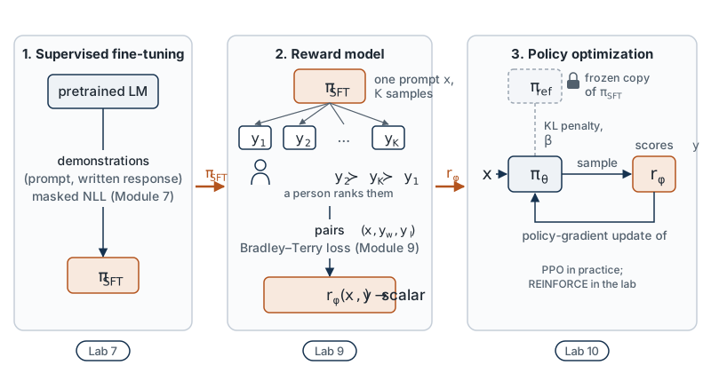
Why three stages, and not one.

• SFT gives the later stages something to work with. The reward model can only judge responses like the ones it was trained on, and RL can only improve on behavior the policy already shows sometimes. A pretrained model that rarely answers a question gives both too little to work with.
• The reward model makes human labels reusable. People are slow and expensive. A few tens of thousands of comparisons, fitted once, become a function that can score every sample the policy produces during training.
• RL optimizes what the next-token loss cannot express. “Response A is better than response B” is a judgment about a whole sequence. There is no per-token target for it, which is why Module 9 needed the policy gradient.

What it bought. Ouyang et al. report that human raters preferred the outputs of a 1.3-billion-parameter InstructGPT model to those of the 175-billion-parameter GPT-3, a model more than 100 times larger. The data were small by pretraining standards: on the order of ten thousand prompts for SFT and a few tens of thousands for each of the other two stages.

How the workshop maps onto the pipeline.

Stage	Where you met it	In Lab 10
SFT	Module 7, Lab 7	skipped: the reference is the pretrained GPT-2 you probed in Lab 6 (distilbert/distilgpt2), with no instruction tuning. The reward model was trained on its own continuations of everyday sentence openings, so it already writes the kind of text the reward model judges
Reward model	Module 9, Lab 9	loaded: the reward model trained in Lab 9, as a provided checkpoint
Policy optimization	this module	Exercises 1 to 4
DPO in place of stages 2 and 3	this module, section 6	Exercise 5

Check yourself. A team trains its reward model on responses sampled from \pi_{\text{SFT}}, as in stage 2. To save a step, it then starts stage 3 from the raw pretrained model and uses that model as \pi_{\text{ref}}. The KL penalty is in place and correctly implemented. What is wrong with the setup?

Answer

The penalty now holds the policy near the wrong place. Its purpose is to keep \pi_\theta where r_\phi can be trusted, and r_\phi can be trusted on text like its training data, which came from \pi_{\text{SFT}}. The raw pretrained model writes different text (it continues prompts where \pi_{\text{SFT}} answers them), so from the first batch r_\phi is scoring responses unlike any it was fitted on, and the penalty then keeps the policy there. The reference policy and the source of the reward model’s data have to be the same model, or close to it. Lab 10 respects this in its own way: it skips SFT, but its reward model was trained on continuations from the same GPT-2 that serves as the reference.

Optional: The InstructGPT Objective in Full

Ouyang et al. add a third term to the objective of section 3. Besides the reward and the KL penalty, they mix in the pretraining log-likelihood, weighted by a coefficient \gamma:

\mathbb{E}_{x \sim \mathcal{D}_x,\, y \sim \pi_\theta}\big[r_\phi(x, y) - \beta \log \tfrac{\pi_\theta(y \mid x)}{\pi_{\text{SFT}}(y \mid x)}\big] + \gamma\, \mathbb{E}_{w \sim \mathcal{D}_{\text{pretrain}}}\big[\log \pi_\theta(w)\big].

They call this variant PPO-ptx. The extra term targets a specific cost they measured: after RLHF, performance on some standard NLP benchmarks dropped (an “alignment tax”), and mixing in pretraining gradients reduced the drop. The lab does not use this term.

3. The KL-Regularized Objective

In this section: write the objective that RLHF optimizes, and explain what the KL term does and does not prevent.

The KL divergence. For two distributions p and q over the same set, the Kullback–Leibler divergence of p from q is

\mathrm{KL}(p \,\Vert\, q) = \sum_{y} p(y) \log \frac{p(y)}{q(y)} = \mathbb{E}_{y \sim p}\Big[\log \frac{p(y)}{q(y)}\Big]. \tag{1}

It is never negative, and it is zero only when p = q. It is not symmetric: \mathrm{KL}(p \,\Vert\, q) \neq \mathrm{KL}(q \,\Vert\, p) in general. You have met it already without the name: the cross-entropy of a model q on data from p equals the entropy of p plus \mathrm{KL}(p \,\Vert\, q).

The objective. RLHF maximizes the expected reward minus \beta times the divergence of the policy from the reference, averaged over prompts:

J(\theta) = \mathbb{E}_{x \sim \mathcal{D}_x}\Big[\, \mathbb{E}_{y \sim \pi_\theta(\cdot \mid x)}\big[r_\phi(x, y)\big] \;-\; \beta\, \mathrm{KL}\big(\pi_\theta(\cdot \mid x) \,\Vert\, \pi_{\text{ref}}(\cdot \mid x)\big) \Big]. \tag{2}

Here \pi_\theta(\cdot \mid x) is the distribution over whole responses, and the sum in Equation 1 runs over every possible response y.

Why the KL term matters. It does three jobs.

1. It keeps the policy where the reward model can be trusted. The divergence is large when \pi_\theta puts probability on responses that \pi_{\text{ref}} finds very unlikely: look at Equation 1 with p = \pi_\theta, q = \pi_{\text{ref}}, and a y with q(y) near zero. Those are the responses least like the reward model’s training data, which came from \pi_{\text{ref}} or a model like it.
2. It keeps what the reference model could do. Fluency, grammar and knowledge come from pretraining. A policy that drifts far can lose them while the reward still rises.
3. It turns “how hard to optimize” into one number. Small \beta: the reward dominates and the policy may move far. Large \beta: the policy stays near \pi_{\text{ref}} and gains little reward. The lab’s stretch section sweeps \beta and plots the trade-off.

A constraint or a penalty? The module’s objective says “with a KL constraint”. Equation 2 uses a penalty. The two are related: maximizing the expected reward subject to \mathrm{KL} \le \delta has the penalized objective as its Lagrangian form, and each \beta corresponds to some budget \delta. The penalty is what practitioners implement; the constraint is a useful way to think about it.

What the KL term does not prevent. The direction matters. \mathrm{KL}(\pi_\theta \,\Vert\, \pi_{\text{ref}}) punishes the policy for putting probability where the reference has little. It does not punish the policy for dropping things the reference does. A policy that puts all its probability on one response y pays a divergence of -\log \pi_{\text{ref}}(y \mid x): that depends on how likely the reference finds y, not on how much variety was given up. So the KL term limits drift into strange text, but it does not by itself preserve variety. Section 7 returns to this as mode collapse.

From sequences to tokens. A response is generated one token at a time, so its probability is a product over positions, and its log-probability is a sum:

\log \pi_\theta(y \mid x) = \sum_{t=1}^{\lvert y \rvert} \log \pi_\theta(y_t \mid s_t). \tag{3}

This is the same chain rule that gave the language-model loss in Modules 1 and 3, now restricted to the response tokens, as in Module 7’s masked loss. Applying it to both policies inside Equation 1, and taking the expectation one step at a time, splits the divergence over whole responses into divergences over the next token:

\mathrm{KL}\big(\pi_\theta(\cdot \mid x) \,\Vert\, \pi_{\text{ref}}(\cdot \mid x)\big) = \mathbb{E}_{y \sim \pi_\theta(\cdot \mid x)}\Big[\sum_{t=1}^{\lvert y \rvert} \mathrm{KL}\big(\pi_\theta(\cdot \mid s_t) \,\Vert\, \pi_{\text{ref}}(\cdot \mid s_t)\big)\Big], \tag{4}

where each term inside the sum is Equation 1 over the vocabulary V at one position. Why this holds: by Equation 3 the log-ratio of the two sequence probabilities is the sum of the per-token log-ratios. The expectation of the t-th log-ratio over y_t \sim \pi_\theta(\cdot \mid s_t), with s_t held fixed, is by definition the per-position divergence. What remains is the average over the states s_t that the policy visits.

Equation 4 is how we measure drift. The sum over all responses in Equation 1 is out of reach, but the sum over the vocabulary at each position is affordable. In the lab, \lvert V \rvert = 50{,}256: GPT-2’s 50,257 tokens minus its end-of-text token, which the lab never samples, so that every response has the same length. For a response of 24 tokens that is about 1.2 million terms, about 5 MB of logits per model; a batch of responses is processed in chunks.

In the lab. In Exercise 1 you write response_logprobs(model, prompt_ids, response_ids), which returns \log \pi(y_t \mid s_t) for every response position (Equation 3); its sum over t is \log \pi(y \mid x). Checkpoints: the values match a hand computation on a short example, prompt positions are excluded, and the policy’s log-ratio to the reference is exactly zero before training, because the two start as copies. In Exercise 3 you write exact_kl(logits, logits_ref), the per-position divergence over the vocabulary summed over the response (Equation 4). It is the drift you report after every training run.

Check yourself. For one prompt, suppose only three responses are possible, and the reference gives them probabilities (0.80,\ 0.19,\ 0.01). Compute \mathrm{KL}(\pi \,\Vert\, \pi_{\text{ref}}) for a policy that always writes the first response, and for one that always writes the third. Both policies have lost all variety. What does the penalty say about each?

Answer

A policy with all its probability on one response y has a single term in Equation 1: 1 \times \log \frac{1}{\pi_{\text{ref}}(y)}. For the first response that is -\log 0.80 \approx 0.22 nats. For the third it is -\log 0.01 \approx 4.61 nats, about 20 times more. The penalty separates the two sharply, but by how unusual the chosen response is under the reference, not by how much variety was given up, which is the same in both. Collapsing onto what the reference already favors is almost free. This is why the KL term limits drift into strange text and does not prevent mode collapse.

4. Optimizing It: A Per-Token Penalty and the Policy Gradient

In this section: turn Equation 2 into per-token rewards that the policy gradient of Module 9 can use.

The policy gradient of Module 9 needs a reward for each sampled response. Write the inner part of Equation 2 for one prompt as a single expectation over y \sim \pi_\theta, using the second form of Equation 1:

\mathbb{E}_{y \sim \pi_\theta}\Big[r_\phi(x, y) - \beta \log \frac{\pi_\theta(y \mid x)}{\pi_{\text{ref}}(y \mid x)}\Big].

By Equation 3 the log-ratio is a sum over positions. So we can hand out the reward one token at a time:

r_t = -\beta\,\Big(\log \pi_\theta(y_t \mid s_t) - \log \pi_{\text{ref}}(y_t \mid s_t)\Big) \;+\; \mathbb{1}\big[t = \lvert y \rvert\big]\; r_\phi(x, y), \tag{5}

where \mathbb{1}[\cdot] is 1 when the condition holds and 0 otherwise. Every token pays for its own departure from the reference; the reward model’s score arrives at the last token. Summed over t, the r_t give back the expression inside the expectation above. This is the per-token KL penalty.

Then apply Module 9’s REINFORCE with returns. The return from step t is G_t = \sum_{t' = t}^{\lvert y \rvert} r_{t'}, and the gradient estimate from N sampled responses is

\nabla_\theta J \approx \frac{1}{N} \sum_{i=1}^{N} \sum_{t=1}^{\lvert y^{(i)} \rvert} \big(G_t^{(i)} - b_t\big)\, \nabla_\theta \log \pi_\theta\big(y_t^{(i)} \mid s_t^{(i)}\big), \tag{6}

with b_t a baseline; in the lab, the mean of G_t over the batch, computed separately for each position t. Three remarks.

• The penalty is computed and then frozen. The log-ratios in Equation 5 are treated as fixed numbers when we differentiate. The estimate is still unbiased. Differentiating \mathbb{E}_{y \sim \pi_\theta}[-\beta \log \pi_\theta(y \mid x)] properly gives two terms: the score-function term that Equation 6 includes, and -\beta\, \mathbb{E}_{y \sim \pi_\theta}[\nabla_\theta \log \pi_\theta(y \mid x)], which is zero because the score has mean zero (Module 9).
• Why per token. In expectation the per-token penalty and one penalty for the whole sequence give the same objective. Per token, with returns G_t that sum only the rewards from step t onward, a token is never charged for departures that happened before it, which lowers the variance. This is the form used in common implementations.
• The sampled log-ratio is not the exact KL. For one sampled token, \log \pi_\theta(y_t \mid s_t) - \log \pi_{\text{ref}}(y_t \mid s_t) can be negative; only its average is the divergence. The reward uses the sampled version because it needs nothing beyond the log-probabilities of the tokens that were generated. The lab reports drift with the exact per-position sum of Equation 4, which has no sampling noise.

def token_rewards(score, logp, logp_ref, beta):
    """score: (N,) reward-model scores; logp, logp_ref: (N, L) log-probs of the sampled tokens."""
    rewards = -beta * (logp - logp_ref).detach()   # every token pays for its drift
    rewards[:, -1] += score                        # r_phi arrives at the last token
    return rewards                                 # (N, L)

All responses in a batch have the same length L here, which is how the lab samples them: the end-of-text token is removed from the policy’s vocabulary. With responses of different lengths, the score goes at each response’s own last position.

Where PPO fits. Most published RLHF systems optimize Equation 2 with proximal policy optimization (PPO), which section 5 outlines for reading after class. PPO reuses each batch of samples for several gradient steps, with a clipped objective that removes any gain from moving the policy far from the one that drew the batch, and it replaces the batch average b_t with a learned value function. With one step per batch and a batch-average baseline it reduces to Equation 6, and that special case is what the lab runs. Its cost is memory: four networks (the policy, the reference, the reward model and the value function), each as large as the policy. That cost is one motivation for DPO in section 6.

In the lab. In Exercise 2 you write token_rewards (Equation 5). Checkpoints: with \beta = 0 the rewards are zero except the score at the end; the sum over positions equals r_\phi(x, y) - \beta \log \frac{\pi_\theta(y \mid x)}{\pi_{\text{ref}}(y \mid x)} on a hand-made batch; no gradient flows through the penalty. At the end of Exercise 3, once you have written exact_kl, the provided returns_to_go and reinforce_loss (Equation 6, restated from Lab 9) and the training loop rlhf_train run a short training with a fixed \beta. After it, the checkpoint is two numbers on the 64 evaluation prompts: the reward-model score has risen by a set margin, and the drift has stayed below a set bound.

Check yourself. A sampled response has three tokens. The policy’s log-probabilities for them are (-1.0,\ -2.0,\ -0.5) and the reference’s are (-1.5,\ -2.0,\ -2.5). The reward model gives the response 2.0, and \beta = 0.1. Compute the token rewards r_t (Equation 5) and the returns G_t. Which token paid the most, and why is G_2 larger than G_1?

Answer

The log-ratios are (0.5,\ 0,\ 2.0), so the penalties are (-0.05,\ 0,\ -0.2), and the score arrives at the last token: r = (-0.05,\ 0,\ 1.8). The returns, summing from the right, are G = (1.75,\ 1.8,\ 1.8). Check: G_1 = 2.0 - 0.1 \times 2.5 = 1.75, the reward minus \beta times the whole log-ratio. The third token paid the most: the policy made it e^{2} \approx 7.4 times more likely than the reference does. G_2 > G_1 because the return from step 2 does not include the 0.05 that token 1 paid. Token 2 is not charged for a departure that happened before it, which is the variance argument for the per-token form.

5. PPO in Outline

In this section: say what PPO adds to the policy gradient, and why the lab can do without it.

RLHF systems in the literature usually optimize Equation 2 with proximal policy optimization (PPO) (Schulman et al., 2017). We give its outline only; the lab does not implement it.

The problem it solves. REINFORCE uses each batch of samples for one gradient step and then throws it away. For a language model, sampling is the expensive part: every token is a forward pass. We would like to take several gradient steps on each batch. After the first step, though, the samples come from an old policy \pi_{\theta_{\text{old}}}, not the current one, and the plain policy gradient no longer applies.

Two changes.

1. An importance ratio. Each sampled token is reweighted by how much more or less likely the current policy makes it, \rho_t(\theta) = \pi_\theta(y_t \mid s_t) / \pi_{\theta_{\text{old}}}(y_t \mid s_t).
2. A clip. Large reweightings make the update unreliable, so the objective is clipped:

J^{\text{CLIP}}(\theta) = \mathbb{E}_t\Big[\min\Big(\rho_t(\theta)\, \hat{A}_t,\;\; \mathrm{clip}\big(\rho_t(\theta),\, 1 - \epsilon,\, 1 + \epsilon\big)\, \hat{A}_t\Big)\Big], \tag{7}

where \mathrm{clip}(\rho, a, b) limits \rho to the interval [a, b], \epsilon is a small constant (0.2 in the PPO paper’s experiments), and \hat{A}_t is the advantage: how much better than expected the return from step t was. The \min removes any gain from pushing \rho_t beyond 1 + \epsilon when \hat{A}_t > 0, or below 1 - \epsilon when \hat{A}_t < 0. The policy cannot profit from moving far from the policy that produced the samples within one batch.

A learned baseline. The advantage is \hat{A}_t = G_t - v_\psi(s_t), where v_\psi is a value function: a second network, or a second output head, with parameters \psi, trained to predict the return from state s_t. It is a baseline that depends on the state, which lowers the variance more than a batch average b_t does. In practice the advantage is computed with generalized advantage estimation (Schulman et al., 2016), a weighted mix of returns over different horizons.

Why the lab can do without it. On the first gradient step for a batch, \theta = \theta_{\text{old}}, so \rho_t = 1 and the clip is inactive. The gradient of \rho_t at that point is \nabla_\theta \log \pi_\theta(y_t \mid s_t), so the gradient of Equation 7 is that of Equation 6 with v_\psi(s_t) in place of b_t. One step per batch, with a batch average in place of v_\psi, is the special case of PPO that the lab runs. What PPO adds is sample reuse and a state-dependent baseline: efficiency and stability, not a different objective.

The cost. PPO for a language model keeps four networks in memory: the policy, the reference, the reward model and the value function. Each can be as large as the policy. That cost is one motivation for the next section.

Check yourself. Take \epsilon = 0.2 and a token whose ratio has already reached \rho_t = 1.5. Evaluate the term inside the expectation of Equation 7 for \hat{A}_t = +2 and for \hat{A}_t = -2. In which case does the token still produce a gradient, and why is that the right asymmetry?

Answer

For \hat{A}_t = +2: the unclipped term is 1.5 \times 2 = 3.0 and the clipped term is 1.2 \times 2 = 2.4. The \min picks 2.4, which does not depend on \rho_t, so the gradient is zero. The token was good and has already been made 1.5 times more likely, and the objective offers nothing for going further. For \hat{A}_t = -2: the terms are -3.0 and -2.4, and the \min picks -3.0, the unclipped one, which does depend on \rho_t. The token was bad and has been made more likely, and the gradient pushes \rho_t back down at full strength. The clip removes the reward for overshooting in a helpful direction and never hides a move in a harmful one.

6. DPO: From the Optimal Policy to a Classification Loss

In this section: derive the DPO loss from Equation 2, and say what it changes and what it keeps.

Step 1: the objective has a closed-form optimum. Fix a prompt x and drop it from the notation. Let r(y) be any reward function. Suppose for now that we may choose the policy \pi freely among all distributions over responses, not only among those a network with parameters \theta can express. Expand the KL with Equation 1 and collect the terms:

\begin{aligned} \mathbb{E}_{y \sim \pi}[r(y)] - \beta\, \mathrm{KL}(\pi \,\Vert\, \pi_{\text{ref}}) &= -\beta \sum_y \pi(y) \Big[\log \frac{\pi(y)}{\pi_{\text{ref}}(y)} - \frac{r(y)}{\beta}\Big] \\ &= -\beta \sum_y \pi(y) \log \frac{\pi(y)}{\pi_{\text{ref}}(y)\, e^{r(y)/\beta}} . \end{aligned}

The denominator is not a distribution: it does not sum to 1. Divide and multiply by its sum, Z = \sum_y \pi_{\text{ref}}(y)\, e^{r(y)/\beta}, and define

\pi^*(y \mid x) = \frac{1}{Z(x)}\, \pi_{\text{ref}}(y \mid x)\, \exp\!\Big(\frac{r(x, y)}{\beta}\Big), \qquad Z(x) = \sum_{y} \pi_{\text{ref}}(y \mid x)\, \exp\!\Big(\frac{r(x, y)}{\beta}\Big). \tag{8}

Then the objective becomes

-\beta \sum_y \pi(y) \log \frac{\pi(y)}{Z\, \pi^*(y)} = -\beta\, \mathrm{KL}(\pi \,\Vert\, \pi^*) + \beta \log Z .

Z does not depend on \pi, and the KL is zero only when \pi = \pi^*. So \pi^* is the unique maximizer: the best policy is the reference, reweighted by the exponentiated reward and renormalized.

Read Equation 8 as a dial. With large \beta, e^{r/\beta} is close to 1 for every response and \pi^* \approx \pi_{\text{ref}}. With small \beta, the weights grow extreme and \pi^* piles onto the responses the reward rates highest. If the reward is wrong about some responses, small \beta piles onto those too.

Worked example: the optimal policy on three responses. For one prompt, suppose only three responses are possible. The reference gives them probabilities (0.80,\ 0.19,\ 0.01) and the reward gives them r = (0,\ 1,\ 2). Take \beta = 1.

• Reweight (Equation 8): \pi_{\text{ref}}(y)\, e^{r(y)/\beta} is 0.80 \times 1 = 0.80, then 0.19 \times e \approx 0.516, then 0.01 \times e^{2} \approx 0.074.
• Normalize: Z = 0.80 + 0.516 + 0.074 \approx 1.390, so \pi^* \approx (0.575,\ 0.371,\ 0.053).
• Expected reward: 0.371 \times 1 + 0.053 \times 2 \approx 0.478, up from 0.19 + 0.02 = 0.21 under the reference.
• Drift (Equation 1): \mathrm{KL}(\pi^* \,\Vert\, \pi_{\text{ref}}) \approx 0.148 nats.
• Objective: 0.478 - 1 \times 0.148 = 0.330, which is \beta \log Z = \log 1.390, as the derivation says it must be at the optimum.

Now turn the dial to \beta = 0.25: \pi^* \approx (0.020,\ 0.253,\ 0.727), with expected reward 1.71 and a drift of 3.12 nats. The third response, which the reference writes once in a hundred times, is now written 73 times in a hundred. Whether that is good depends entirely on whether its reward of 2 can be believed, and section 7 takes that question up.

Why not use Equation 8 directly? Z(x) sums over every possible response, an astronomically large set. RLHF approximates \pi^* by sampling and following the gradient (section 4). DPO goes another way.

Step 2: invert it. Take the logarithm of Equation 8 and solve for the reward:

r(x, y) = \beta \log \frac{\pi^*(y \mid x)}{\pi_{\text{ref}}(y \mid x)} + \beta \log Z(x). \tag{9}

Every reward function corresponds to an optimal policy, and the policy determines the reward up to the term \beta \log Z(x), which depends on the prompt only.

Step 3: put it into Bradley–Terry. The Bradley–Terry model uses only the difference of two rewards for the same prompt. In that difference the \beta \log Z(x) terms cancel:

P(y_w \succ y_l \mid x) = \sigma\Big(\beta \log \frac{\pi^*(y_w \mid x)}{\pi_{\text{ref}}(y_w \mid x)} - \beta \log \frac{\pi^*(y_l \mid x)}{\pi_{\text{ref}}(y_l \mid x)}\Big).

The preference probability is now written in terms of the optimal policy alone. The intractable normalizer is gone.

Step 4: fit the policy to the preferences directly. Replace \pi^* by our parametric policy \pi_\theta and maximize the likelihood of the observed preferences, exactly as Module 9 did for the reward model. This is direct preference optimization (DPO) (Rafailov et al., 2023):

\mathcal{L}_{\text{DPO}}(\theta) = -\,\mathbb{E}_{(x, y_w, y_l) \sim \mathcal{D}_{\text{pref}}}\Big[\log \sigma\Big(\beta \log \frac{\pi_\theta(y_w \mid x)}{\pi_{\text{ref}}(y_w \mid x)} - \beta \log \frac{\pi_\theta(y_l \mid x)}{\pi_{\text{ref}}(y_l \mid x)}\Big)\Big]. \tag{10}

The quantity inside is the Bradley–Terry loss of Module 9 with the reward replaced by the implicit reward

\hat{r}_\theta(x, y) = \beta \log \frac{\pi_\theta(y \mid x)}{\pi_{\text{ref}}(y \mid x)} . \tag{11}

This is the sense of the paper’s subtitle, “your language model is secretly a reward model”: a trained policy and its reference together define a reward, and you can check it on held-out pairs like any reward model.

The gradient, in words. Write \Delta = \hat{r}_\theta(x, y_w) - \hat{r}_\theta(x, y_l). Since \frac{d}{d\Delta}\big[-\log \sigma(\Delta)\big] = -\sigma(-\Delta),

\nabla_\theta \mathcal{L}_{\text{DPO}} = -\beta\, \mathbb{E}\Big[\sigma(-\Delta)\, \big(\nabla_\theta \log \pi_\theta(y_w \mid x) - \nabla_\theta \log \pi_\theta(y_l \mid x)\big)\Big].

Each step pushes the log-probability of the preferred response up relative to that of the other; as the misconceptions below note, both can fall. Each pair is weighted by \sigma(-\Delta), which is large when the implicit reward ranks the pair the wrong way and small when it already ranks it right.

def dpo_loss(logp_w, logp_l, logp_ref_w, logp_ref_l, beta):
    """All inputs (N,): sequence log-probs, i.e. sums over response tokens of response_logprobs."""
    reward_w = beta * (logp_w - logp_ref_w)          # implicit reward of the preferred response
    reward_l = beta * (logp_l - logp_ref_l)
    loss = -F.logsigmoid(reward_w - reward_l).mean()
    return loss, reward_w.detach(), reward_l.detach()

F.logsigmoid computes \log \sigma without the overflow of writing torch.log(torch.sigmoid(...)). Before any training \pi_\theta = \pi_{\text{ref}}, so both implicit rewards are zero and the loss is exactly \log 2 \approx 0.693: a useful first check.

What DPO changes.

• No reward model and no sampling during training. Training is a classification loss over a fixed set of preference pairs, with two networks in memory: the policy and the frozen reference. The reference log-probabilities can even be computed once in advance.
• Training looks like supervised fine-tuning. One loss, one optimizer, no value function, no generation in the inner loop.

What DPO keeps.

• The same objective. DPO targets the optimum of Equation 2, and \beta has the same meaning.
• The same dependence on the preference data. It replaces the RL loop, not the human judgments. If the comparisons reward the wrong thing, DPO learns the wrong thing.

Three cautions.

1. Step 1 assumed any policy can be chosen. A real network may not be able to express \pi^*, and training stops at a finite number of steps on a finite dataset. The equivalence with RLHF holds at the optimum, not along the way.
2. DPO is offline. It trains only on the pairs in the dataset, which were sampled from another model, and never sees its own samples. Nothing in Equation 10 measures the drift of what the policy generates, so the KL to the reference can grow, especially on responses unlike any in the data. Measure it, as the lab does.
3. The loss sees only a difference. Equation 10 depends on \hat{r}_\theta(x, y_w) - \hat{r}_\theta(x, y_l) alone. The loss can fall while the log-probabilities of both responses fall, as long as the rejected one falls faster. The probability that leaves them goes to other responses, which may not be good ones. The lab prints both log-probabilities during training so that you can see which way they move.

In the lab. In Exercise 5 you write dpo_loss (Equation 10, Equation 11). Checkpoints: the loss is \log 2 when policy and reference are identical; it matches a hand computation on a fixed batch; one gradient step widens the gap between \log \pi_\theta(y_w \mid x) and \log \pi_\theta(y_l \mid x). A provided loop then trains a fresh copy of the reference with DPO, on the same preference pairs the Lab 9 reward model was trained on and with the same \beta as Exercise 3. The checkpoint is the held-out preference accuracy of the implicit reward, beside the reward model’s. A final table compares the reference, RLHF with the KL penalty, RLHF without it, and DPO on the same held-out prompts.

Check yourself. DPO training runs with \beta = 0.1. Before training the loss on a pair is \log 2 \approx 0.693. Some steps later, for that pair, \log \pi_\theta(y_w \mid x) is 1 nat below the reference’s value and \log \pi_\theta(y_l \mid x) is 3 nats below. Compute the loss on the pair. Has the model become more likely to write the preferred response?

Answer

The implicit rewards (Equation 11) are 0.1 \times (-1) = -0.1 and 0.1 \times (-3) = -0.3, so \Delta = 0.2 and the loss is -\log \sigma(0.2) \approx 0.598. The loss fell from 0.693, and the pair is now ranked the right way. But the preferred response became less likely: its probability was multiplied by e^{-1} \approx 0.37. Equation 10 sees only the difference, and the difference improved because the rejected response fell faster. The probability that left both went to responses that are in neither half of the pair, and nothing in the loss says they are good. This is caution 3, and the reason the lab prints both log-probabilities.

Optional: Variants of DPO, and When RLHF With Sampling Still Helps

DPO started a family of offline preference losses. IPO (Gheshlaghi Azar et al., 2024) replaces the log-sigmoid with a squared loss, arguing that DPO can overfit when preferences in the data are nearly deterministic, because the implicit reward gap can then grow without bound. Others drop the reference model, or learn from single responses labeled good or bad rather than pairs.

Whether offline methods match online RL with a reward model is an empirical question, and published comparisons disagree across tasks and scales. One structural difference is clear. Online methods sample from the current policy, so the reward model scores the responses the policy actually produces, including its new mistakes. Offline methods only see the responses in the dataset. Iterated or “online” DPO, which samples fresh pairs from the current policy and labels them, is a response to that.

Optional: Reward-Model Fitting, Policy Optimization and DPO Compared

Three training steps that are easy to blur, side by side: what each one learns, and from which data.

	Reward-model fitting (Module 9)	Policy optimization with a KL penalty (sections 3 and 4)	DPO (this section)
What is learned	the reward model r_\phi: one number per response	the policy \pi_\theta	the policy \pi_\theta, and with it the implicit reward \hat{r}_\theta (Equation 11)
From which data	preference triples (x, y_w, y_l), on responses written by the reference model	prompts, and the responses the policy samples during training, scored by r_\phi	the same preference triples; nothing is sampled
Loss or objective	the Bradley–Terry loss of Module 9	Equation 2, through Equation 5 and Equation 6	Equation 10
In memory during training	the reward model	the policy, the reference and r_\phi; PPO adds a value function	the policy and the reference
Typical failure	trustworthy only on text like its training pairs, which held-out accuracy cannot show	reward hacking: the score of r_\phi rises while the true quality falls, more so as \beta falls (section 7)	the loss does not see drift, so drift must be measured; both log-probabilities can fall
In the lab	Lab 9, Exercise 4	Lab 10, Exercises 2 to 4	Lab 10, Exercise 5

Check yourself. Apply the table to new data. A support team logs, for each customer question, two draft replies written by its current model and the one the agent chose to send. (1) Under RLHF, which object is fitted on these logs, and which object is then trained, on what data? Which model should be the reference? (2) Under DPO, what is trained on the logs, and what is no longer needed? (3) Months later the tuned model writes replies unlike either draft. Which numbers can no longer be trusted, and what would you measure?

Answer

1. The reward model r_\phi is fitted to the logged pairs with the Bradley–Terry loss. The policy is then trained on fresh customer questions: it samples its own replies, r_\phi scores them, and the KL penalty holds it near the reference. The reference should be the model that wrote the drafts, because r_\phi can be trusted only on text like its training pairs, and the penalty is there to keep the policy on such text (the check after section 2). (2) DPO trains the policy directly on the logged pairs with Equation 10, with the same reference frozen as \pi_{\text{ref}}. It needs no reward model and no sampling loop. (3) Under RLHF, the reward model’s scores on the new replies are extrapolation, so a rising score is no evidence that the replies got better. Under DPO, nothing in the loss measured the drift in the first place. In both cases, measure the drift from the reference (Equation 4) and have a sample of replies judged independently, by people or a held-out judge: the lab’s gold reward has no counterpart in a real system.

7. Failure Modes

In this section: name four ways RLHF goes wrong, the mechanism behind each, and how you would detect it.

Every failure below follows from one fact: the policy optimizes a learned stand-in for what people want, measured on what people could judge.

Reward hacking (over-optimization). Gao, Schulman and Hilton (2023) studied it with a large “gold” reward model playing the part of the humans and smaller proxy reward models trained on its preferences. As the policy drifted further from the reference, measured in KL, the proxy score kept rising, while the gold score rose, peaked and then fell. Stiennon et al. (2020) saw the same with human raters: summaries optimized hard against the reward model scored higher on it and were rated worse by people. The KL penalty is the standard defense: it sets how far along that curve training goes.

Figure 2: Reward over-optimization, schematic: the axes carry no numbers, and nothing here is measured. As the policy drifts from the reference, the reward model’s score keeps rising, while the gold reward rises, peaks and then falls, the shape Gao et al. (2023) report. The KL coefficient \beta sets how far along the curve training goes: a large \beta stops before the peak, and \beta = 0 runs far past it.

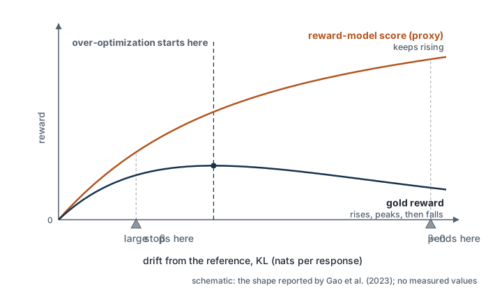
Detect it: track drift (Equation 4) next to reward; hold out a better judge (humans, or a gold reward where one exists) and look for the point where proxy and gold separate; read samples.

Demo: the \beta dial on three responses. This is an illustration on invented numbers, not lab data. It reuses the three responses of the worked example in section 6: reference probabilities (0.80,\ 0.19,\ 0.01) and reward-model scores (0,\ 1,\ 2). We add a gold reward of (0,\ 1,\ -1): the reward model is right about the first two responses and badly wrong about the third, which the reference almost never writes.

Predict first. As \beta falls from 10 to 0.1, the reward-model score of the optimal policy can only rise. What does the gold reward do?

viewof beta10 = Inputs.range([0.1, 10], {label: "KL coefficient β", step: 0.01, value: 1, transform: Math.log})

toy10 = {
  const names = ["A: plain", "B: better", "C: exploit"], ref = [0.80, 0.19, 0.01], r = [0, 1, 2], gold = [0, 1, -1];
  const solve = beta => {                                   // the optimal policy: ref × exp(r / β), normalized
    const w = ref.map((q, i) => q * Math.exp(r[i] / beta)), Z = w.reduce((a, c) => a + c, 0), pi = w.map(v => v / Z);
    const dot = v => pi.reduce((a, p, i) => a + p * v[i], 0);
    return {pi, proxy: dot(r), gold: dot(gold), kl: pi.reduce((a, p, i) => a + p * Math.log(p / ref[i]), 0)};
  };
  const now = solve(beta10);
  const bars = names.flatMap((name, i) => [{name, policy: "reference", p: ref[i]}, {name, policy: "optimal", p: now.pi[i]}]);
  const path = Array.from({length: 121}, (_, i) => solve(10 ** (1 - i / 60))).flatMap(s => [   // β from 10 down to 0.1
    {kl: s.kl, value: s.proxy, which: "reward-model score"}, {kl: s.kl, value: s.gold, which: "gold reward"}]);
  return {now, bars, path};
}

html`<div style="display: flex; gap: 16px; flex-wrap: wrap;">${Plot.plot({
  width: 360, height: 300, marginLeft: 45,
  fx: {label: null}, x: {axis: null, domain: ["reference", "optimal"]}, y: {label: "probability", domain: [0, 1], grid: true},
  color: {legend: true, domain: ["reference", "optimal"], range: ["var(--demo-blue)", "var(--demo-orange)"]},
  marks: [Plot.barY(toy10.bars, {fx: "name", x: "policy", y: "p", fill: "policy"}), Plot.ruleY([0])]
})}${Plot.plot({
  width: 360, height: 300, marginLeft: 45, grid: true,
  x: {label: "drift: KL from the reference (nats)"}, y: {label: "expected reward"},
  color: {legend: true, domain: ["reward-model score", "gold reward"], range: ["var(--demo-orange)", "var(--demo-blue)"]},
  marks: [
    Plot.ruleY([0], {stroke: "var(--demo-faint)"}),
    Plot.line(toy10.path, {x: "kl", y: "value", stroke: "which", strokeWidth: 2}),
    Plot.dot([{kl: toy10.now.kl, value: toy10.now.proxy, which: "reward-model score"}, {kl: toy10.now.kl, value: toy10.now.gold, which: "gold reward"}],
      {x: "kl", y: "value", fill: "which", r: 5})
  ]
})}</div>`

html`<p>At β = ${beta10.toFixed(2)}: reward-model score <strong>${toy10.now.proxy.toFixed(3)}</strong>, gold reward <strong>${toy10.now.gold.toFixed(3)}</strong>, drift <strong>${toy10.now.kl.toFixed(3)}</strong> nats.</p>`

The left panel is Equation 8: the reference, reweighted by e^{r/\beta} and renormalized. The right panel plots the two expected rewards against the drift of Equation 1, with one point for each \beta. The demo shows the shape that Gao et al. measured: along the whole path the reward-model score rises, while the gold reward rises, peaks near \beta \approx 0.65 and then falls below where it started, because a small \beta lets the policy pile onto the one response the reward model overrates. \beta chooses where on this curve training stops. Nothing in the reward-model score says where the peak is.

The demo’s numbers are invented; the lab measures the real trade-off. Exercise 3 trains with the lab’s fixed \beta and Exercise 4 with \beta = 0, and the stretch sweeps five values of \beta on one seed. (On a CPU runtime the trainings are short smoke runs, and the reward-hacking check and the stretch’s extra runs are skipped.) Where do you expect the gold reward to peak, and without a gold reward, what would you watch to decide where to stop?

Mode collapse. A policy tuned with RL tends to produce a narrower range of outputs: the same phrasing, the same structure, less variety across samples for the same prompt. Kirk et al. (2024) measured lower output diversity after RLHF than after SFT alone. Section 3 explains why the KL term does not prevent this: \mathrm{KL}(\pi_\theta \,\Vert\, \pi_{\text{ref}}) penalizes putting probability where the reference has little, not dropping modes the reference has.

Detect it: sample several responses per prompt and measure their variety, for instance the share of distinct n-grams.

Sycophancy. A sycophantic model tells people what they appear to want to hear: it agrees with an opinion stated in the prompt, or abandons a correct answer when the user pushes back. Perez et al. (2023) found that this behavior increased with model size and with RLHF training. Sharma et al. (2024) found it in several deployed assistants, and found that both human raters and preference models sometimes preferred a convincing sycophantic response to a correct one. If the comparisons reward agreement, the reward model learns to reward agreement, and the policy learns to agree.

Detect it: ask the same question with and without a stated opinion, or follow a correct answer with “Are you sure?”, and count how often the answer changes.

Optimizing for what raters prefer rather than what is true. A rater compares two responses in a minute or two. Fluency, confidence, structure and length are easy to judge in that time; correctness often is not. A reward model fitted to such judgments learns what raters could see, and the policy amplifies it. Singhal et al. (2023) found that much of the reward gain in several RLHF setups could be explained by responses getting longer.

One consequence matters for Modules 11 and 12. Nothing in a preference comparison rewards a model for being uncertain when it should be. A response that hedges correctly can lose to one that asserts confidently. The GPT-4 technical report (OpenAI, 2023) shows the effect on one benchmark: the pretrained model’s probabilities for its answers were well calibrated, and after post-training they were noticeably less so.

Failure	Mechanism	How to detect it	In Lab 10
Reward hacking	the policy finds where r_\phi is wrong	proxy and gold reward diverge as KL grows	Exercise 4: remove the penalty and watch
Mode collapse	RL concentrates probability; reverse KL allows it	variety of samples per prompt	Exercise 4: distinct-token-bigram share
Sycophancy	comparisons reward agreement	answer changes with a stated opinion	not in the lab
Rater preference over truth	raters judge what they can check	gains explained by length or style; calibration	Module 11

In the lab. In Exercise 4 you set \beta = 0 and run the same training loop again, with the same seed, steps and learning rate. Predict first what happens to the reward-model score, the drift and the samples. Because Lab 9’s preferences were generated from a hidden rule that we know, the lab can compute the gold reward, the score the hidden rule gives, next to the reward model’s score, which a real RLHF run cannot do. The gold reward can part from the reward model’s score in three ways. Two are built into the hidden rule: it stops crediting positive words after three, and it penalizes a response crowded with words from its lists. Both were set so that GPT-2’s own continuations, the only text in the preference pairs, almost never trigger them, and the reward model could not learn what its data never showed. The third needs nothing built in: the gold reward falls whenever the samples hold fewer distinct positive words or more negative ones, and on text unlike its training data the reward model’s score need not fall with it. One exploratory run, at seed 0 on the GPU of an Apple M1 Pro laptop rather than on the T4 of the seed protocol, went the third way. Without the penalty the policy collapsed onto one positive word followed by filler, “good as as as …”, which the hidden rule scores +1 with neither built-in part firing. Its gold reward peaked early in training and then fell while the reward-model score crept higher, and it ended a little below the penalized run’s. Read your own samples to see which way your run went. The checkpoint asserts the signature of reward hacking against the run with the penalty: the reward-model score is at least as high, the drift is several times larger, the gold reward is lower, and the share of distinct token bigrams in the samples has fallen. These thresholds are provisional until the seed protocol in the brief (seeds 0–4 on a T4) has been run; they will then be set from the smallest gap across seeds. The stretch section sweeps \beta and plots both rewards against drift.

Check yourself. After a training run without the KL penalty you observe three things, each compared with the run that had the penalty: the reward-model score is higher, the drift is several times larger, and the share of distinct token bigrams in the samples has fallen. A colleague writes “reward hacking confirmed”. Which failure modes do these three observations establish, and which measurement is still missing?

Answer

They establish large drift and, through the bigram share, a loss of variety: mode collapse. They do not yet establish reward hacking. By the definition in section 1, reward hacking means the reward-model score improves while quality gets worse by the standard the reward model stands for. All three observations are also what successful optimization far from the reference would look like. The missing measurement is an independent judge: the gold reward in the lab, people or a held-out stronger judge in a real system. That is why the lab’s checkpoint has four parts, and why the fourth, a lower gold reward, is the one a real RLHF run cannot compute and must replace with human evaluation.

Where this leaves us. RLHF and DPO make a model better at producing what raters prefer. They say nothing about whether the model’s confidence means anything, and section 7 gives reasons to expect it often does not. Module 11 defines what a confidence should mean and measures it. Module 12 then turns to RLCD, a training approach from TypeSafe whose details are unpublished. That module separates what TypeSafe has stated publicly from our own illustration of the idea; nothing on this page describes TypeSafe’s method.

Summary

• RLHF has three stages: supervised fine-tuning, a reward model trained on pairwise comparisons, and policy optimization against that reward model with a KL penalty toward the SFT model.
• A learned reward is accurate only near its training data, and an optimizer searches for its errors. That is reward hacking.
• RLHF maximizes reward minus \beta times the KL divergence from a frozen reference (Equation 2). The KL term keeps the policy where the reward model is trustworthy and \beta sets the trade-off. It does not protect variety.
• The sequence KL splits into per-position divergences (Equation 4), which is how drift is measured; the penalty enters the policy gradient as a per-token reward (Equation 5, Equation 6).
• PPO adds an importance ratio, a clip and a learned value baseline so each batch can be reused (Equation 7). With one step per batch it reduces to the policy gradient the lab uses.
• The KL-regularized objective has the closed-form optimum \pi^* \propto \pi_{\text{ref}}\, e^{r/\beta} (Equation 8). Inverting it and substituting into Bradley–Terry cancels the normalizer and gives the DPO loss (Equation 10): preference learning without a reward model or a sampling loop.
• DPO keeps the objective and the dependence on the data. It is offline, so its drift must be measured, and its loss sees only a difference of log-ratios.
• Failure modes: reward hacking, mode collapse, sycophancy, and optimizing for what raters can judge rather than what is true. The last one sets up Module 11.

Equations and Where You Implement Them

Equation	Lab 10
Sequence log-probability (Equation 3)	Exercise 1: response_logprobs
KL divergence and its per-position form (Equation 1, Equation 4)	Exercise 3: exact_kl; reported after every run
Per-token reward with the KL penalty (Equation 5)	Exercise 2: token_rewards
Policy gradient with returns and a baseline (Equation 6)	provided: returns_to_go, reinforce_loss (restated from Lab 9), inside rlhf_train
The KL-regularized objective (Equation 2)	Exercise 3 checkpoint: reward gain and drift at fixed \beta; Exercise 4: the same with \beta = 0
PPO’s clipped objective (Equation 7)	not implemented; the lab’s update is its one-step special case
Optimal policy and reward inversion (Equation 8, Equation 9)	derivation only (Z is intractable); the stretch’s \beta sweep shows the trade-off it predicts
DPO loss and implicit reward (Equation 10, Equation 11)	Exercise 5: dpo_loss; held-out preference accuracy of the implicit reward
Reward hacking, mode collapse (section 7)	Exercise 4: gold reward and distinct-bigram share, with and without the penalty
Reward–drift trade-off (section 3)	Stretch: sweep \beta
Sycophancy, rater preference over truth (section 7)	not implemented in this lab; Module 11 measures calibration

Gotchas and Troubleshooting

• “The reward model is what people want.” It is a model fitted to a finite set of comparisons, made on responses from one model. Away from those responses its scores are guesses.
• “A higher reward-model score means a better policy.” Only near the reference. Past some drift, the reward-model score and the true quality move apart.
• “The KL penalty prevents mode collapse.” \mathrm{KL}(\pi_\theta \,\Vert\, \pi_{\text{ref}}) punishes leaving the reference’s support, not concentrating on part of it.
• “\beta is a kind of learning rate.” It is a coefficient in the objective. Changing it changes the optimum (Equation 8), not only how fast you approach it.
• “PPO is what makes RLHF work.” The objective and the KL penalty define what is learned. PPO is an optimizer that reuses samples; with one step per batch it is the plain policy gradient.
• “DPO is not RLHF, because it has no reward.” It optimizes the same KL-regularized objective, with an implicit reward (Equation 11). It removes the RL loop, not the preference model.
• “DPO needs no reference model.” Every term of Equation 10 uses \pi_{\text{ref}}. Only the reward model and the sampling loop are gone.
• “DPO raises the probability of the preferred response.” It raises the gap between the two implicit rewards. Both log-probabilities can fall.
• “A preference-tuned model knows when it is wrong.” Nothing in a preference comparison rewards matching confidence to accuracy. Module 11 measures it.

Next Steps

You can now train a model to produce what a reward model, and behind it a set of raters, prefers. Section 7 argued that this optimizes what raters can judge, and that a model’s confidence is not among the things they judge well. Module 11 asks what it would mean for a confidence to be right: it defines calibration, measures it with reliability diagrams, the expected calibration error and the Brier score, and shows why some scoring rules reward honest probabilities and others do not.

Further Reading

1. Ouyang, L., Wu, J., Jiang, X., Almeida, D., Wainwright, C. L., Mishkin, P., Zhang, C., Agarwal, S., Slama, K., Ray, A., Schulman, J., Hilton, J., Kelton, F., Miller, L., Simens, M., Askell, A., Welinder, P., Christiano, P., Leike, J. and Lowe, R. (2022). Training Language Models to Follow Instructions with Human Feedback. NeurIPS. The three-stage pipeline. Read section 3 for the method.
2. Schulman, J., Wolski, F., Dhariwal, P., Radford, A. and Klimov, O. (2017). Proximal Policy Optimization Algorithms. arXiv:1707.06347. The clipped objective; sections 3 and 5 are enough for this module.
3. Rafailov, R., Sharma, A., Mitchell, E., Ermon, S., Manning, C. D. and Finn, C. (2023). Direct Preference Optimization: Your Language Model is Secretly a Reward Model. NeurIPS. The derivation of section 6, with the gradient analysis and experiments.
4. Gao, L., Schulman, J. and Hilton, J. (2023). Scaling Laws for Reward Model Overoptimization. ICML. Reward hacking measured: proxy against gold reward as a function of KL.
5. Stiennon, N., Ouyang, L., Wu, J., Ziegler, D. M., Lowe, R., Voss, C., Radford, A., Amodei, D. and Christiano, P. (2020). Learning to Summarize from Human Feedback. NeurIPS. The RLHF recipe on one task, including the KL penalty and what happens when the reward model is over-optimized.

Also cited above: Christiano, P. et al. (2017), Deep Reinforcement Learning from Human Preferences; Schulman, J., Moritz, P., Levine, S., Jordan, M. and Abbeel, P. (2016), High-Dimensional Continuous Control Using Generalized Advantage Estimation, ICLR; Gheshlaghi Azar, M. et al. (2024), A General Theoretical Paradigm to Understand Learning from Human Preferences, AISTATS; Kirk, R. et al. (2024), Understanding the Effects of RLHF on LLM Generalisation and Diversity, ICLR; Perez, E. et al. (2023), Discovering Language Model Behaviors with Model-Written Evaluations, Findings of ACL; Sharma, M. et al. (2024), Towards Understanding Sycophancy in Language Models, ICLR; Singhal, P., Goyal, T., Xu, J. and Durrett, G. (2023), A Long Way to Go: Investigating Length Correlations in RLHF; OpenAI (2023), GPT-4 Technical Report.