Seq2seq and Attention

Day 1 · Foundations Module 4 95 minutes (45 briefing, 50 lab) 15:25 briefing · 16:10 lab

Encoder-decoder models, the fixed-vector bottleneck, and attention as the fix.

Open the lab in Colab PyTorch

Duration: 95 minutes (45 briefing, 50 lab)
Level: 300 · Advanced
Lab runtime: Google Colab, free T4 GPU · about 10 minutes of compute
Accounts and cost: Google. Free
Without API keys: the lab always runs its real models

What You Will Build

In this module you will:

Assemble an encoder-decoder’s teacher-forced forward pass and loss
Explain the fixed-vector bottleneck and measure it by input length
Implement dot-product and additive attention and read attention maps against the expected alignment

New terms, in the glossary: attention.

Before You Start

Module 3 · Sequence Models and its lab, and the modules before it: this module measures its results against theirs.
A Google account, and the Colab runtime set to T4 GPU (Runtime → Change runtime type).
No API keys: the lab runs its own models throughout.

Where we are. Module 3’s recurrent language model reads a prefix of any length and emits one prediction per input token, in step with it. It has no way to map one sequence to another, of a different length and in a different order: a sentence to its translation, a written date to ISO format. This module asks one question: how should the source reach the model that writes the target, and what breaks when it has to pass through a single vector?

In the Lab

Open the lab in Colab

5 exercises in 3 parts. The notebook budgets 47 minutes for them; the lab slot is 50 minutes. Each exercise you write is a # TODO stub with a folded solution beneath it and a checkpoint that passes or fails; where people tend to stall, a folded hint sits above the stub.

Task	Briefing section	Time
Part A · The Encoder-Decoder Without Attention
Exercise 1 · Teacher-Forced Forward Pass and Loss	2	10 min
Exercise 2 · Exact Match by Input Length	3	8 min
Part B · Attention
Exercise 3 · Dot-Product Attention	4, 5	12 min
Exercise 4 · The Additive Score	5	10 min
Part C · Reading Attention
Exercise 5 · Attention Heat-Maps and the Alignment Hit Rate	6	7 min

Challenge · Beam Search

Optional, for anyone who finishes the core path early: the notebook’s stretch section, after the last checkpoint.

When you are done. Runtime → Disconnect and delete runtime releases the machine; your keys stay in Colab Secrets for the next lab.

Agenda

Minutes	Section	In the room
0–5	1. From Next-Token Prediction to Transduction	—
5–13	2. The Encoder-Decoder Model	—
13–19	3. The Fixed-Vector Bottleneck	Check yourself (2 min)
19–35	4. Attention	Demo (4 min)
35–40	5. Three Score Functions	—
40–45	6. Attention as Soft Alignment	Check yourself (2 min)
45	Total	37 minutes of exposition, 8 of activities

Checks, demos and predictions listed here are part of the live session and its minutes; the others on the page are for reading afterwards.

Read now · Sections 1–6, in the agenda above.

Use in the lab · Exercise 1: section 2; Exercise 2: section 3; Exercise 3: sections 4 and 5; Exercise 4: section 5; Exercise 5: section 6.

Read later · Section 7, Decoding (Reference); section 8, Attention as a Query-Key-Value Lookup (Reference); the collapsed callouts marked Optional or After the Lab; Further Reading.

Section 8 is not taught here because Module 5 opens Day 2 with the same material, live: its section 1 restates attention as a query-key-value lookup and asks the two questions that end this page.

1. From Next-Token Prediction to Transduction

In this section: state what Module 3’s language model cannot do as it stands.

Module 3 built a recurrent language model. It reads a prefix w_1, \dots, w_{t-1}, keeps a hidden state h_{t-1}, and outputs a distribution over the next token w_t. Input and output are the same sequence, shifted by one position.

Many tasks do not have that shape. Translation, summarization, and the date normalization used in Lab 4 map one sequence to another sequence:

Source: x_1, \dots, x_S, with length S.
Target: y_1, \dots, y_T, with length T.

In general S \neq T, and the tokens do not line up one to one. The input 3 March 2021 has 12 characters; its output 2021-03-03 has 10, and the year moves from the end to the front. A model that emits one output per input step cannot do this. This kind of task is called sequence transduction, and a model for it is a sequence-to-sequence (seq2seq) model.

We want a model of the conditional probability of the target given the source. The chain rule of probability factorizes it exactly, one target token at a time:

P_\theta(y_1, \dots, y_T \mid x_1, \dots, x_S) = \prod_{t=1}^{T} P_\theta(y_t \mid y_1, \dots, y_{t-1}, x_1, \dots, x_S). \tag{1}

Here \theta denotes all model parameters. Each factor is a next-token prediction, as in Module 3, with one addition: it is also conditioned on the whole source. So a seq2seq model is a conditional language model. The only new question is how the source gets in.

2. The Encoder-Decoder Model

In this section: write down the encoder, the decoder, and the training loss.

The answer of Sutskever et al. (2014) and Cho et al. (2014) uses two recurrent networks.

The encoder reads the source. Let e_{x_i} \in \mathbb{R}^d be the embedding of source token x_i. The encoder produces one hidden state per source position:

h_i = \mathrm{RNN}_{\mathrm{enc}}(h_{i-1}, e_{x_i}), \qquad i = 1, \dots, S, \qquad h_0 = 0. \tag{2}

\mathrm{RNN}_{\mathrm{enc}} is any recurrent cell from Module 3 (the lab uses a GRU), and h_i \in \mathbb{R}^{d_h}, where d_h is the hidden size. If the cell is an LSTM, its cell state is carried along as well; we omit it from the notation.

The decoder is a second recurrent network with its own parameters. We write its states as s_t \in \mathbb{R}^{d_h} to keep them apart from the encoder states h_i. It starts from the encoder’s final state and then runs as a language model over the target:

s_0 = h_S, \qquad s_t = \mathrm{RNN}_{\mathrm{dec}}(s_{t-1}, e_{y_{t-1}}), \qquad t = 1, \dots, T. \tag{3}

The input at step t is the embedding of the previous target token y_{t-1}. Two special tokens mark the boundaries: y_0 is a start token <bos>, and the target ends with an end token <eos>, so that the model can decide when to stop.

The output layer turns each decoder state into a distribution over the target vocabulary V:

z_t = W_o s_t + b_o, \qquad P_\theta(y_t \mid y_{<t}, x) = \mathrm{softmax}(z_t), \tag{4}

where z_t \in \mathbb{R}^{|V|} are the logits, W_o \in \mathbb{R}^{|V| \times d_h} and b_o \in \mathbb{R}^{|V|} are the output weights and bias, y_{<t} abbreviates y_1, \dots, y_{t-1}, and x abbreviates the whole source.

The loss is the negative log-likelihood of the correct target. Taking -\log of Equation 1 turns the product into a sum:

\mathcal{L}(\theta) = -\sum_{t=1}^{T} \log P_\theta(y_t \mid y_{<t}, x). \tag{5}

This is the cross-entropy loss of Module 3, summed over target positions. Gradients flow from the loss through the decoder, through s_0 = h_S, and into the encoder, so both networks are trained together.

Teacher forcing. During training the decoder input at step t is the correct previous token y_{t-1}, not the model’s own prediction, exactly as in Module 3. At test time the correct target is unknown, so the decoder feeds its own output back in (section 7).

In code, as in the lab. tgt_in is the target shifted right (it starts with <bos>) and tgt_out is the target itself (it ends with <eos>), so position t of tgt_in holds y_{t-1} and position t of tgt_out holds y_t:

def forward_plain(model, src, src_len, tgt_in):
    h, h_S = model.encode(src, src_len)                        # h: (B, S, d_h), unused here
    s, _ = model.dec(model.tgt_emb(tgt_in), h_S.unsqueeze(0))  # s_0 = h_S; s: (B, T, d_h)
    return model.W_o(s)                                        # z_t = W_o s_t + b_o: (B, T, |V|)

def seq2seq_loss(logits, tgt_out):                             # -log P(y_t | y_<t, x), averaged
    return F.cross_entropy(logits.reshape(-1, logits.size(-1)), tgt_out.reshape(-1),
                           ignore_index=PAD)                   # padding positions are skipped

The lab averages the loss over the non-padding target tokens of a batch instead of summing it as in Equation 5. The average is the sum divided by the number of target tokens in the batch, which does not depend on \theta, so it has the same minimizer.

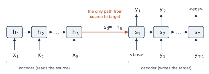
An encoder reads the source into a single vector that initializes the decoder. — Figure 1: The encoder-decoder model. The encoder states h_1, \dots, h_S read the source and the decoder states s_1, \dots, s_T write the target. The initial decoder state s_0 = h_S is the only path from source to target.

In the lab. The encoder (Equation 2), the decoder cell and the training loop are provided. In Exercise 1 you write forward_plain and seq2seq_loss: the teacher-forced forward pass and the loss of Equation 3, Equation 4 and Equation 5. The checkpoint asks for an untrained loss close to \ln |V| = \ln 15 \approx 2.71 nats per token.

Check yourself. The target is 2021-03-03, one character per token, followed by <eos>. How many factors does Equation 1 have for it? For an untrained model over the lab’s 15 target tokens, what is the summed loss Equation 5, and what does the lab’s averaged loss print? Under teacher forcing, the model predicts 7 at step 2 where the target has 0. What is the decoder’s input at step 3?

Answer

Eleven factors: ten characters and <eos>, which the model must also predict so that it knows when to stop. An untrained model is close to uniform, so each factor costs about \ln 15 = 2.71 nats: the sum is about 11 \times 2.71 = 29.8 nats and the average is 2.71. The average is the number the checkpoint tests, because it does not depend on the target’s length. At step 3 the input is the embedding of 0, the correct y_2. Teacher forcing feeds the true previous token whatever the model predicted, which is why all eleven losses come from a single forward pass.

3. The Fixed-Vector Bottleneck

In this section: explain why this model degrades as the source gets longer.

Look at where the source enters Equation 3: only through s_0 = h_S. Everything the decoder will ever know about the source is contained in that one vector. Formally, the model’s prediction depends on x only through h_S:

P_\theta(y_1, \dots, y_T \mid x_1, \dots, x_S) = P_\theta(y_1, \dots, y_T \mid h_S).

The vector h_S has d_h dimensions whether the source has 5 tokens or 500. The amount of information to be carried grows with S; the size of the container does not. This is the fixed-vector bottleneck.

Two further things make it worse in practice:

The encoder must decide what to keep before it knows what will be asked. It compresses the source once, and the decoder cannot go back and look again.
The path is long. The first source token influences the last target token through S + T recurrent steps. Module 3 showed that gradients shrink along such paths. Gating (LSTM, GRU) helps but does not remove the problem.

These are two different problems. The first is about capacity: even a perfectly trained model cannot fit an unbounded amount of information in d_h numbers. The second is about optimization. Attention addresses both.

Optional: The Evidence From Translation

The evidence is empirical. Bahdanau et al. (2015) report that the translation quality of the fixed-vector model drops quickly as sentences get longer. Sutskever et al. (2014) found that simply reversing the source sentence helped markedly, because it shortens the path between the first source words and the first target words. A trick like that is a sign that the architecture is fighting the task.

In the lab. The source contains K dates, K = 1 to 4, so the amount the decoder must remember grows with the input. In Exercise 2 you write exact_match (the whole output string must be right) and measure it by K for the model without attention. What it scores in each bucket is the lab’s prediction; the result is in the box after the lab.

After the Lab: What Lab 4 Measured in Exercise 2

Open this after Exercise 2, so that it does not answer the lab’s prediction for you. At the lab’s budget (d_h = 128, 4,000 training steps) the model without attention breaks as soon as a second date appears: exact match is 0.898 for one date and 0.000 for two, three and four. It keeps only the first date. In every bucket the first output date is right for 0.90 to 0.93 of the sources and every later date for none, although the outputs still have the right number of well-formed ISO dates. More capacity or training would raise these numbers. The claim is about an equal budget, which the attention model of section 4 gets.

Check yourself. Double the source length from S to 2S and leave the target alone. In the plain encoder-decoder, how do these two quantities change: the number of values in the vector that carries the source to the decoder, and the number of recurrent steps between the first source token and the last target token? Which of the two problems named above does each belong to?

Answer

The vector does not change: h_S has d_h values whatever S is, so twice the information must fit in the same space. That is the capacity problem. The path grows from S + T steps to 2S + T, so the gradient that tells the encoder how to store the first token passes through S more recurrent steps. That is the optimization problem, the one Module 3 analyzed. A longer source makes both worse at once, which is why they are easy to confuse. They have different cures, though: a larger d_h addresses capacity and does nothing for the path, while gating helps the path and leaves capacity alone.

4. Attention

In this section: derive the attention step, from scores to weights to the context vector.

The idea. Keep all encoder states h_1, \dots, h_S, not just the last. At each decoder step, let the decoder choose which of them to read.

Choosing a single state (a hard choice) is not differentiable, so we cannot train it with backpropagation. We take a weighted average instead, with weights that the model computes. This takes three steps at each decoder step t.

Step 1: score. A score function compares the current decoder state with each encoder state and returns a real number, larger when h_i is more relevant to what the decoder needs now:

\mathrm{score}(s_t, h_i) \in \mathbb{R}, \qquad i = 1, \dots, S.

Section 5 gives three choices for this function. For now, take the simplest: the dot product s_t^\top h_i.

Step 2: normalize. A softmax over the source positions turns the S scores into weights:

\alpha_{t,i} = \frac{\exp\big(\mathrm{score}(s_t, h_i)\big)}{\sum_{j=1}^{S} \exp\big(\mathrm{score}(s_t, h_j)\big)}. \tag{6}

By construction \alpha_{t,i} > 0 and \sum_{i=1}^{S} \alpha_{t,i} = 1. The attention weight \alpha_{t,i} is how much target step t reads from source position i. Note that this softmax runs over the S source positions. It is not the softmax over the vocabulary in Equation 4.

A worked example with S = 3: scores (2, 0, 0) give \exp values (7.39, 1, 1), which sum to 9.39, so the weights are (0.79, 0.11, 0.11). The largest score dominates, but the others still contribute.

Step 3: average. The context vector is the weighted average of the encoder states:

\bar{h}_t = \sum_{i=1}^{S} \alpha_{t,i}\, h_i . \tag{7}

Worked example: one attention step with vectors. Take S = 3 and d_h = 2, with encoder states h_1 = (1, 0), h_2 = (0, 1), h_3 = (-1, 0) and decoder state s_t = (2, 0).

Score with the dot product: s_t^\top h_1 = 2, s_t^\top h_2 = 0, s_t^\top h_3 = -2.
Normalize (Equation 6): the exponentials are (7.389,\ 1,\ 0.135), with sum 8.524, so \alpha_t = (0.867,\ 0.117,\ 0.016).
Average (Equation 7): \bar{h}_t = 0.867\,(1, 0) + 0.117\,(0, 1) + 0.016\,(-1, 0) = (0.851,\ 0.117).

The context is mostly h_1, the state that points the same way as the query, but it is not h_1: every state contributes. Now suppose position 3 is padding, a filler position that makes the sources of a batch equally long (see Padding below). Its score is set to -\infty, its exponential is 0, and the softmax runs over the other two: \alpha_t = (0.881,\ 0.119,\ 0) and \bar{h}_t = (0.881,\ 0.119). The weights of the real positions rise so that the row still sums to one.

Notation. The original papers write the context vector as c_t. In this workshop c_t is the LSTM cell state from Module 3, so we write the context as \bar{h}_t: the bar is a reminder that it is an average of encoder states h_i. It lives in the same space, \bar{h}_t \in \mathbb{R}^{d_h}.

Using the context. The decoder now has two vectors at step t: its own state s_t (what it has produced so far) and the context \bar{h}_t (what it just read from the source). We concatenate them, written [s_t; \bar{h}_t] \in \mathbb{R}^{2 d_h}, and pass them through one layer to obtain the attentional state \tilde{s}_t, which replaces s_t in the output layer:

\tilde{s}_t = \tanh\big(W_c\, [s_t; \bar{h}_t] + b_c\big), \qquad z_t = W_o \tilde{s}_t + b_o, \tag{8}

with W_c \in \mathbb{R}^{d_h \times 2 d_h} and b_c \in \mathbb{R}^{d_h}. The rest is unchanged: \mathrm{softmax}(z_t) gives the distribution over y_t, and the loss is still Equation 5.

Why this fixes the bottleneck.

Capacity. The decoder reads from S vectors, so the memory grows with the source. A different context \bar{h}_t is computed at every step, so nothing has to be decided in advance.
Path length. Each h_i is connected to each output step through Equation 7 in a single step, however far apart they are. Gradients no longer have to survive S + T recurrent steps.
Trainability. Every operation in Equation 6, Equation 7 and Equation 8 is differentiable. The attention weights are not supervised; they are learned from the ordinary loss, because reading the right source position lowers it.

What it costs. One score per pair of target and source positions: S \times T score evaluations per sequence pair, where the plain model needed none.

Padding. In a batch, shorter sources are padded to a common length. Padded positions must receive zero weight. We achieve this by setting their scores to -\infty before the softmax, since \exp(-\infty) = 0.

In code, for all T decoder steps of a batch at once. The step after the score is shared by every score function, so it is a function of its own:

def masked_attention(scores, keys, mask):  # scores: (B, T, S), keys: (B, S, d_h), mask: (B, S)
    scores = scores.masked_fill(~mask.unsqueeze(1), float("-inf"))  # padding: exp(-inf) = 0
    alpha = torch.softmax(scores, dim=-1)  # softmax over the S source positions: (B, T, S)
    h_bar = alpha @ keys                   # sum_i alpha_ti h_i: (B, T, d_h)
    return alpha, h_bar

def dot_product_attention(q, keys, mask):  # q: (B, T, d_h), the decoder states s_t
    return masked_attention(q @ keys.transpose(1, 2), keys, mask)  # scores s_t^T h_i

In the lab. Exercise 3 is the attention step, in the two functions above: masked_attention(scores, keys, mask) (the masked softmax of Equation 6 and the context vector of Equation 7) and dot_product_attention(q, keys, mask) (the scores of Equation 9). Both return (alpha, h_bar). The combination layer of Equation 8 is provided. The attention model is trained with the same d_h, steps, optimizer and batches as the plain model; its exact match by K is in the box after the lab.

After the Lab: What Lab 4 Measured With Attention

Open this after the lab has trained the attention model, so that it does not answer the lab’s prediction for you. Trained with the same d_h, steps, optimizer and batches as the plain model, the attention model reaches exact match 1.000 for every K from 1 to 4, where the plain model scored 0.000 from K = 2 on.

Try it: turn the query, watch the weights. Five encoder states h_1, \dots, h_5 are placed by hand in two dimensions. You control the decoder state s_t, the query: its direction and its length. The demo computes dot-product scores s_t^\top h_i, the weights \alpha_{t,i} of Equation 6 and the context vector \bar{h}_t of Equation 7. This is an illustration, not states from Lab 4.

Predict first. The query starts out pointing nearest to h_1. Double its length without turning it. Do the weights become more peaked, flatter, or stay the same? Then try to find a query that puts the context vector \bar{h}_t outside the pentagon formed by the five states.

viewof qAngle = Inputs.range([0, 360], {value: 20, step: 1, label: "Direction of the query (degrees)"})
viewof qLen = Inputs.range([0, 3], {value: 1.5, step: 0.1, label: "Length of the query"})

{
  const keys = [[1.4, 0.15], [0.7, 1.25], [-0.85, 1.1], [-1.4, -0.3], [0.3, -1.4]]
    .map(([x, y], i) => ({x, y, name: "h" + "₁₂₃₄₅"[i]}));
  const rad = qAngle * Math.PI / 180, q = {x: qLen * Math.cos(rad), y: qLen * Math.sin(rad)};
  const scores = keys.map((h) => q.x * h.x + q.y * h.y);                 // s_t^T h_i
  const top = Math.max(...scores), ex = scores.map((s) => Math.exp(s - top));
  const total = ex.reduce((a, b) => a + b, 0);
  const rows = keys.map((h, i) => ({...h, score: scores[i], alpha: ex[i] / total}));   // softmax over positions
  const ctx = {x: rows.reduce((a, d) => a + d.alpha * d.x, 0), y: rows.reduce((a, d) => a + d.alpha * d.y, 0)};
  const plane = Plot.plot({
    width: 360, height: 360, grid: true,
    x: {domain: [-3.4, 3.4], label: "dimension 1"}, y: {domain: [-3.4, 3.4], label: "dimension 2"},
    marks: [
      Plot.line([...rows, rows[0]], {x: "x", y: "y", stroke: "var(--demo-faint)", strokeDasharray: "3 3"}),
      Plot.arrow(rows, {x1: 0, y1: 0, x2: "x", y2: "y", stroke: "var(--demo-blue)", strokeWidth: 2, strokeOpacity: (d) => 0.25 + 0.75 * d.alpha}),
      Plot.text(rows, {x: (d) => 1.18 * d.x, y: (d) => 1.18 * d.y, text: "name", fontSize: 13, fill: "var(--demo-blue)"}),
      Plot.arrow([q], {x1: 0, y1: 0, x2: "x", y2: "y", stroke: "var(--demo-ink)", strokeWidth: 2.5}),
      Plot.text([q], {x: (d) => d.x + 0.45 * Math.cos(rad), y: (d) => d.y + 0.45 * Math.sin(rad), text: () => "query", fontSize: 13, fontWeight: "bold"}),
      Plot.dot([ctx], {x: "x", y: "y", r: 6, fill: "var(--demo-orange)"})
    ]
  });
  const bars = Plot.plot({
    width: 360, height: 360, marginBottom: 40,
    x: {label: "source position", domain: rows.map((d) => d.name)}, y: {label: "attention weight α", domain: [0, 1]},
    marks: [
      Plot.barY(rows, {x: "name", y: "alpha", fill: "var(--demo-blue)"}),
      Plot.text(rows, {x: "name", y: "alpha", text: (d) => d.alpha.toFixed(2), dy: -8}),
      Plot.ruleY([0])
    ]
  });
  return html`<div style="display:flex;flex-wrap:wrap;gap:1.5rem;align-items:flex-end">${plane}${bars}</div>
  <p>Scores: (${scores.map((s) => s.toFixed(2)).join(", ")}). Context vector (orange dot): (${ctx.x.toFixed(2)}, ${ctx.y.toFixed(2)}).</p>`;
}

The direction of the query decides which state gets the most weight; its length decides how much. Lengthening the query multiplies every score by the same factor, which widens the gaps between them, and the softmax sharpens. At length 0 every score is 0, the weights are uniform, and the context is the plain mean of the states. The orange dot never leaves the pentagon: the weights are positive and sum to one, so \bar{h}_t is always a blend of the states and never one state exactly.

Check yourself. The scores (2, 0, 0) gave the weights (0.79, 0.11, 0.11). Without computing any exponentials, what are the weights for the scores (12, 10, 10)? Are the weights for (20, 0, 0) more or less peaked than (0.79, 0.11, 0.11)? What is the context vector when all S scores are equal?

Answer

(12, 10, 10) gives the same weights, (0.79, 0.11, 0.11). Adding a constant to every score multiplies the numerator and the denominator of Equation 6 by the same factor, so only the differences between scores matter. (20, 0, 0) is far more peaked: the gap grew from 2 to 20, the ratio of weights from e^2 \approx 7 to e^{20} \approx 5 \times 10^8, and the first weight is 1 to eight decimal places. Equal scores give \alpha_{t,i} = 1/S for every i, and the context is the plain average of the encoder states. Attention with equal scores is the order-blind averaging of Module 2. It selects something only once training has moved the scores apart.

Optional: Where Exactly Does the Context Enter the Decoder?

The two founding papers differ in the order of operations.

Luong et al. (2015), followed above: run the decoder cell first to get s_t, attend with s_t as the query, then combine s_t and \bar{h}_t just before the output layer (Equation 8).
Bahdanau et al. (2015): attend with the previous state s_{t-1} as the query, then feed the context into the recurrent cell as an extra input, s_t = \mathrm{RNN}_{\mathrm{dec}}(s_{t-1}, [e_{y_{t-1}}; \bar{h}_t]).

Bahdanau et al. also use a bidirectional encoder: one RNN reads the source left to right, another right to left, and h_i is the concatenation of their two states at position i, so that each h_i summarizes the context on both sides.

We use the Luong ordering because the query is then simply the current decoder state, which makes the step to Module 5 cleaner. The weights and the context vector are computed by the same equations in both versions.

5. Three Score Functions

In this section: write the dot-product, general and additive scores and say when each applies.

The score function is the only part of attention that has design freedom. Three choices are standard.

Dot product (Luong et al., 2015):

\mathrm{score}(s_t, h_i) = s_t^\top h_i . \tag{9}

It has no parameters and is the cheapest to compute. It requires s_t and h_i to have the same dimension, and it forces the decoder and encoder to use the same coordinates for “relevant”.

General, also called multiplicative or bilinear (Luong et al., 2015):

\mathrm{score}(s_t, h_i) = s_t^\top W_a h_i , \tag{10}

with a learned matrix W_a. The matrix lets the two states have different dimensions and lets the model learn which directions of s_t should match which directions of h_i. The dot product is the special case W_a = I (the identity matrix).

Additive (Bahdanau et al., 2015):

\mathrm{score}(s_t, h_i) = u^\top \tanh\big(W_q s_t + W_k h_i\big). \tag{11}

Read it from the inside out. W_q \in \mathbb{R}^{d_a \times d_h} and W_k \in \mathbb{R}^{d_a \times d_h} project the decoder state and the encoder state into a shared space of dimension d_a (the attention size). The projections are added, which is where the name comes from. The \tanh is applied elementwise, and the learned vector u \in \mathbb{R}^{d_a} reduces the result to a single number. This is a feed-forward network with one hidden layer, as in Module 2, applied to the pair (s_t, h_i).

Score	Parameters	Needs equal dimensions	Cost per pair
Dot product	none	yes	one dot product
General	W_a	no	one matrix-vector product
Additive	W_q, W_k, u	no	a one-hidden-layer network

Neither family is uniformly better; Luong et al. (2015) compare them on translation and find the result depends on the setup. Multiplicative scores are cheaper because they reduce to matrix products over all pairs at once. Module 5 keeps the multiplicative form for that reason.

The additive score in code. Each projection is computed once, and broadcasting forms all T \times S sums:

def additive_score(q, keys, W_q, W_k, u):   # q: (B, T, d_h), keys: (B, S, d_h)
    q_proj = (q @ W_q.T).unsqueeze(2)       # W_q s_t: (B, T, 1, d_a)
    k_proj = (keys @ W_k.T).unsqueeze(1)    # W_k h_i: (B, 1, S, d_a)
    return torch.tanh(q_proj + k_proj) @ u  # u^T tanh(W_q s_t + W_k h_i): (B, T, S)

The sum q_proj + k_proj holds B \times T \times S \times d_a numbers, where the dot product needs only the B \times T \times S scores. That is the cost in the last column of the table.

In the lab. Exercise 3 uses the dot-product score (Equation 9). In Exercise 4 you write additive_score(q, keys, W_q, W_k, u) (Equation 11) and pass its scores to the same masked_attention. The checkpoint compares your scores with the equation evaluated one pair at a time. Training a model with the additive score is optional and off by default, because it would be a third training run. The general score (Equation 10) is not implemented in the lab.

Check yourself. Take d_h = 128 and attention size d_a = 64. How many parameters does each of the three scores add to the model? For a batch with B = 64, T = 11 and S = 40, how many numbers does additive_score hold just before the \tanh, and how many scores come out?

Answer

Dot product: none. General: W_a is 128 \times 128 = 16{,}384. Additive: W_q and W_k are 64 \times 128 each and u has 64 entries, 2 \times 8{,}192 + 64 = 16{,}448. So the two learned scores cost about the same in parameters. They differ in computation. The additive score forms q_proj + k_proj, with B \times T \times S \times d_a = 64 \times 11 \times 40 \times 64 = 1{,}802{,}240 numbers, to produce B \times T \times S = 28{,}160 scores: d_a = 64 intermediate numbers per score. The multiplicative scores get each score from one matrix product with no intermediate of that size, which is the reason Module 5 keeps the multiplicative form.

6. Attention as Soft Alignment

In this section: read an attention heat-map and state what it does and does not show.

Collect the weights into a matrix with one row per target position and one column per source position, so that entry (t, i) is \alpha_{t,i}. Each row sums to one. Plotted as a heat-map, this matrix shows where the decoder was reading when it produced each output token.

In statistical machine translation, an alignment records which source word each target word translates. Attention computes a soft alignment: a distribution over source positions instead of a single link. It is learned without any alignment labels.

For the date task the expected pattern is easy to state. While the decoder writes the four digits of the year, the weight should sit on the year in the source, wherever it is. While it writes the month digits 03, the weight should sit on the word March. When the source and target order differ, the bright cells leave the diagonal. Exercise 5 plots this map for 3 March 2021 from the lab’s trained model; the recorded run’s map is in the box after the lab, below.

Two cautions when reading these maps:

The weights show where the model read, not why. A bright cell says that h_i contributed strongly to \bar{h}_t. It does not explain how that information was used.
h_i is not the token x_i. Each encoder state summarizes the source up to position i (or around it, with a bidirectional encoder). The weight can therefore land one position away from where you expect.

In the lab. In Exercise 5 you plot the matrix of \alpha_{t,i} for 3 March 2021 and three test inputs, then write alignment_hit_rate(alphas, examples, tol): the share of target digits whose largest weight lies inside the span of the correct date, or at most tol positions after it.

After the Lab: What Lab 4 Measured in Exercise 5

Open this after Exercise 5, so that it does not answer the lab’s prediction for you.

Heat-map of measured attention weights. Columns are the 12 characters of 3 March 2021, rows are the output characters 2021-03-03 and the end token. Most rows have a single dark cell holding almost all the weight: the year rows on the digits of 2021 at the right, the month rows on and just after the word March, the day rows on the 3 and the space after it at the left. The dark cells therefore run against the diagonal. 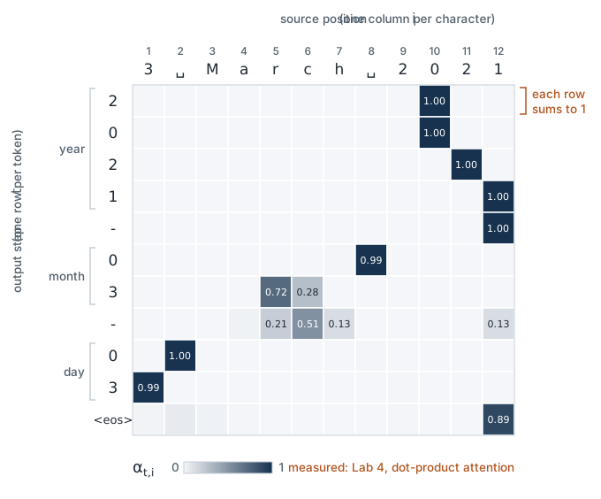— Figure 2: Attention weights \alpha_{t,i} measured in Lab 4 for the source `3 March 2021` (columns) and the model’s output `2021-03-03`, followed by `<eos>` (rows). Dot-product attention model of the recorded run, greedy decoding; the output is correct. Each row sums to 1. Weights of at least 0.10 are printed, rounded to two decimals. Data: `data/lab04_attention_example.json`; drawn by `scripts/make_figures_04.py`.

Figure 2 shows the expected pattern, measured. Most rows are close to one-hot: 8 of the 11 rows put more than 0.99 of their weight on a single position. The year rows read the year, the month rows read March and the day rows read 3. But the weight often lands on a neighbor of the character you would point to. The first digit of the year, 2, is read at the source 0 after it. The month’s 0 is read at the space after March, and its 3 mostly at r, the first letter at which Mar can no longer be May. The day’s leading 0 is read at the space after 3: that is the first state at which the encoder has seen that the day has a single digit and so needs a leading zero.

Both cautions above show in this map. The day’s leading zero has a plausible reason; for the first year digit the map alone gives none. In the lab’s unidirectional encoder the weight often lands one position away from where you expect, as the figure shows.

On the test set, with tol = 1 to allow for the unidirectional encoder, alignment_hit_rate is 0.996; an arg-max drawn uniformly over the source would score between 0.23 and 0.41 for K \ge 2. The off-by-one shifts mostly stay inside the date: with tol = 0 the rate is still 0.99 or more in every bucket.

Check yourself. The source is 12 May 2020 and the encoder reads left to right, so h_i has seen characters 1 to i and nothing after them. The decoder must write the month as 05. What is the first source position whose state can settle which month it is? If a month row of the heat-map put all its weight on the M, what could the decoder learn from it?

Answer

Position 6, the y. The characters are 1, 2, space, M, a, y. After M the month could be March or May; after Ma it still could. Only h_6 has read enough to rule out March. A row with all its weight on the M would return h_4, a state computed before the month was decided. It could tell the decoder that a month starting with M is here, not which one. So you should expect the month rows to read at the y or just after it, not before. Where Lab 4’s month rows read for March is in the box after the lab, above. A bright cell marks the state that was read, and a state knows only its prefix.

7. Decoding

In this section: distinguish greedy decoding from beam search.

At test time we want a target sequence with high probability under Equation 1. Searching all sequences is infeasible: there are |V|^T of them.

Greedy decoding picks the most probable token at each step, \arg\max_{w \in V} P_\theta(w \mid y_{<t}, x), where y_{<t} now holds the tokens the model has already chosen. It feeds the chosen token back as the next input and stops at <eos>. It is fast, and it is what the lab’s core path uses. It can miss the best sequence, because the best first token does not always start the best sequence.

Beam search keeps the B best partial outputs at every step instead of one, where B is the beam size. It is still approximate, but it explores more. B = 1 is greedy decoding.

Whether the extra search helps depends on the model. Beam search earns its cost when the model is uncertain between several outputs, as in translation. Whether it helps on the date task is the prediction of the lab’s stretch section; the result is in the box after the lab, below.

Module 3’s sampling strategies (temperature, top-k, nucleus) are the alternative when variety is wanted. For transduction tasks with one correct answer, such as dates, we want the most probable output, so we search.

Check yourself. A model with a two-token vocabulary \{a, b\} gives the first token the probabilities P(a) = 0.6, P(b) = 0.4. After a, its most probable continuation has probability 0.5. After b, its most probable continuation has probability 0.9. Which two-token output does greedy decoding return, and with what probability? Which does beam search with B = 2 return?

Answer

Greedy takes a, because 0.6 > 0.4, and then the best continuation: probability 0.6 \times 0.5 = 0.30. Beam search with B = 2 keeps both first tokens alive, extends each, and compares complete outputs: 0.30 for the best output starting with a against 0.4 \times 0.9 = 0.36 for the best starting with b. It returns the second. The best first token did not start the best sequence. Greedy can never recover from that, because it has discarded b before seeing what follows. How close the first choice is on the lab’s date model is what the stretch section’s comparison shows.

Optional: Beam Search in Detail

A hypothesis is a partial output y_1, \dots, y_t together with its log-probability so far, which we call its value (to keep the word “score” for attention):

\log P_\theta(y_1, \dots, y_t \mid x) = \sum_{\tau=1}^{t} \log P_\theta(y_\tau \mid y_{<\tau}, x).

The algorithm:

Start with one hypothesis, <bos>, with value 0.
Extend each of the B current hypotheses by every token in V. This gives B \times |V| candidates, each valued by adding the new token’s log-probability.
Keep the B candidates with the highest values.
A hypothesis that ends in <eos> is finished: set it aside and continue with the rest.
Stop at a maximum length or when enough hypotheses have finished. Return the finished hypothesis with the best value.

Length normalization. Every added token contributes a negative log-probability, so longer hypotheses have lower values and raw beam search prefers short outputs. The usual correction is to compare finished hypotheses by value divided by length.

Cost. Each step runs the decoder on B hypotheses, so beam search costs about B times as much as greedy decoding.

No guarantee. Beam search does not always return the most probable sequence, and a larger beam does not always give a better output by the task metric.

The stretch section of the lab implements this algorithm as beam_search(model, source, B), which returns the output string and its log-probability, and checks that B = 1 reproduces greedy decoding exactly. It then compares B = 1, 3, 5 on 200 test sources; the result is in the box after the lab.

After the Lab: What Lab 4 Measured With Beam Search

Open this after the lab’s stretch section, so that it does not answer its prediction for you. On the date task beam search changes nothing: the attention model puts almost all its probability on one output, so greedy decoding already finds it. Compared on 200 test sources, B = 1, 3, 5 tie: exact match 1.000 and mean log-probability -0.0007 for all three beam sizes. On the lab’s date model the first choice is almost never as close as in the check above, which is why the two decoders tie there.

8. Attention as a Query-Key-Value Lookup

In this section: restate attention in the general form that Module 5 builds on.

Nothing in section 4 depends on the vectors coming from an RNN. Rename the parts:

The query q is the vector that asks. Here q = s_t.
The keys k_1, \dots, k_S are what the query is compared against.
The values v_1, \dots, v_S are what is returned.

In seq2seq attention the encoder states play both roles: k_i = v_i = h_i. The attention step, with the target index dropped, is then

\alpha_i = \frac{\exp\big(\mathrm{score}(q, k_i)\big)}{\sum_{j} \exp\big(\mathrm{score}(q, k_j)\big)}, \qquad \mathrm{output} = \sum_{i} \alpha_i\, v_i . \tag{12}

Compare this with a dictionary lookup. A dictionary returns the one value whose key equals the query. Attention is a soft lookup: it returns a blend of all the values, weighted by how well each key matches the query.

General form	In this module
query q	decoder state s_t
keys k_i	encoder states h_i
values v_i	encoder states h_i
weights \alpha_i	\alpha_{t,i}
output	context vector \bar{h}_t

The additive score already hints that queries and keys can be given separate learned projections: W_q acts on the query and W_k on the keys.

The question for Day 2. Our model still has two recurrent networks, and recurrence is sequential: h_i cannot be computed before h_{i-1}, so the positions of a sequence cannot be processed in parallel. But attention already connects any two positions in one step. So:

What if a sequence attends to itself, with queries, keys and values all taken from the same sequence?
What if we then drop the recurrence altogether?

That is the transformer, and it is where Module 5 starts.

Check yourself. Try the first question now. Let a sequence attend to itself with this module’s dot-product score, taking q = k_i = v_i = h_i directly from the states. Suppose all the states have the same length \lVert h_i \rVert. For the query q = h_t, which position gets the highest score? What does that suggest is missing?

Answer

Position t itself. The score is h_t^\top h_i = \lVert h_t \rVert\, \lVert h_i \rVert \cos(h_t, h_i), and with equal lengths it is largest where the cosine is 1, which is at i = t. Each position would mostly read itself and learn nothing new. The score also cannot be asymmetric: h_t^\top h_i = h_i^\top h_t, so if a verb attends to its subject, the subject must attend equally (before normalization) to the verb. What is missing is a way for a position to ask for something different from what it is. Module 5 supplies it by giving the query, the key and the value each their own learned projection of h_i, the step that this module’s additive score already took for W_q and W_k.

Summary

A seq2seq model is a conditional language model: it factorizes P_\theta(y \mid x) over target positions (Equation 1) and is trained with cross-entropy under teacher forcing (Equation 5).
The plain encoder-decoder passes the source to the decoder through one vector, s_0 = h_S. Its size is fixed while the source grows: the fixed-vector bottleneck.
Attention keeps all encoder states. At each target step it scores them against the decoder state, normalizes the scores with a softmax over source positions (Equation 6), and averages (Equation 7).
The score can be a dot product (Equation 9), a bilinear form (Equation 10) or a small network (Equation 11).
The weights \alpha_{t,i} form a soft alignment that can be plotted and inspected.
Greedy decoding takes the best token at each step; beam search keeps B hypotheses. Both are approximate, and whether beam search helps depends on how confident the model is.
Attention is a soft lookup with a query, keys and values (Equation 12). Here q = s_t and k_i = v_i = h_i.

Equations and Where You Implement Them

Equation	Lab 4
Decoder, output layer and loss (Equation 3, Equation 4, Equation 5)	Exercise 1: `forward_plain(model, src, src_len, tgt_in)`, `seq2seq_loss(logits, tgt_out)`
The bottleneck, measured	Exercise 2: `exact_match(preds, golds)`, then exact match by K
Weights and context with the padding mask (Equation 6, Equation 7)	Exercise 3: `masked_attention(scores, keys, mask)`
Dot-product score (Equation 9)	Exercise 3: `dot_product_attention(q, keys, mask)`, returns `(alpha, h_bar)`
Additive score (Equation 11)	Exercise 4: `additive_score(q, keys, W_q, W_k, u)`, passed to `masked_attention`
The matrix of \alpha_{t,i} as a heat-map	Exercise 5: `plot_attention` (provided) and `alignment_hit_rate(alphas, examples, tol)`
Beam search	Stretch: `beam_search(model, source, B)`
Encoder, combination layer, greedy decoding (Equation 2, Equation 8, section 7)	provided: `Seq2Seq.encode`, `readout`, `greedy_decode`
General score (Equation 10)	not implemented

Gotchas and Troubleshooting

“Attention replaces the RNN.” Not in this module. Here attention is added to a recurrent encoder and decoder. Removing the recurrence is Module 5’s step.
“The bottleneck is the vanishing-gradient problem again.” They are different. Vanishing gradients are an optimization problem on long paths. The bottleneck is a capacity problem: a fixed-size vector cannot hold an unbounded amount of information, however well it is trained.
“Attention picks one source token.” It computes a weighted average over all of them. The weights are often peaked (in Lab 4 most rows put more than 0.99 on one position), but they are never exactly zero or one.
“The softmax in attention is over the vocabulary.” It is over the S source positions. The softmax over the vocabulary comes later, in the output layer.
“Attention weights explain the model’s decision.” They show which encoder states were read, not how the information was used. Treat a heat-map as evidence, not as an explanation.
“Attention is trained with alignment labels.” There are none. The weights are learned from the same cross-entropy loss as everything else.
“Beam search finds the most probable output.” It finds a good one. It is a heuristic search, and a wider beam is not guaranteed to do better on the task metric.