Retrieval-Augmented Generation

Day 4 · Calibration, Decisions, RAG Module 13 120 minutes (55 briefing, 55 lab, 10 debrief) 14:45 briefing · 15:40 lab · 16:35 debrief

Building a RAG pipeline with LlamaIndex and LangChain, and evaluating retrieval and answers separately.

Open the lab in Colab LlamaIndex LangChain Jev

Duration: 120 minutes (55 briefing, 55 lab, 10 debrief)
Level: 300 · Advanced
Lab runtime: Google Colab, free T4 GPU · about 8 minutes of compute
Accounts and cost: Google; optional: OpenAI, Anthropic, TypeSafe. Free without keys. Keyed run: under 50 cents on Claude, under 5 cents on OpenAI, under 5 cents on Jev (estimates)
Without API keys: an open model runs in place of the commercial one

What You Will Build

In this module you will:

Assemble a RAG pipeline in LlamaIndex and LangChain
Implement recall@k and MRR, and choose chunk size and top-k from a measured sweep
Evaluate retrieval and answer quality separately

New terms, in the glossary: retrieval, recall@k, reranking, faithfulness.

Before You Start

Module 12 · Calibrated Decisions: RLCD and Jev and its lab, and the modules before it: this module measures its results against theirs.
A Google account, and the Colab runtime set to T4 GPU (Runtime → Change runtime type).
API keys are optional. Without them an open model runs in place of the commercial one.

Module 12 ended with a decision model that answers typed questions about a state, and with thresholds that turn its probabilities into actions. A decision, like a generated answer, is only as good as the text in front of the model, and nothing so far chooses that text. This module answers two questions: how do we put the right passages in front of a model, and when an answer is wrong, how do we tell whether the passages or the model failed?

In the Lab

Open the lab in Colab

6 exercises in 2 parts. The notebook budgets 48 minutes for them; the lab slot is 55 minutes. Each exercise you write is a # TODO stub with a folded solution beneath it and a checkpoint that passes or fails; where people tend to stall, a folded hint sits above the stub.

Task	Briefing section	Time
Exercise 0 · What You Have	2, 8	4 min
Part A · Measuring Retrieval
Exercise 1 · Recall@k and Reciprocal Rank	8	8 min
Exercise 2 · Build the Index, Then Choose L and k at a Fixed Budget	3, 4	9 min
Exercise 3 · The Same Retriever in LangChain	4, 11	8 min
Part B · Reranking and Answers
Exercise 4 · Rerank the Candidates	6	9 min
Exercise 5 · Faithfulness	7, 9	10 min

Challenge · Hybrid Retrieval With BM25

Optional, for anyone who finishes the core path early: the notebook’s stretch section, after the last checkpoint.

When you are done. Runtime → Disconnect and delete runtime releases the machine; your keys stay in Colab Secrets for the next lab.

Agenda

Minutes	Section	In the room
0–3	1. What Module 12 Left Open: Why Retrieve	—
3–8	2. The Pipeline	Check yourself (2 min)
8–12	3. Chunking	—
12–18	4. Dense Retrieval	—
18–22	5. Sparse and Hybrid Retrieval	—
22–30	6. Reranking: Cross-Encoders and a Decision Model	Check yourself (2 min)
30–33	7. Generation: Sources, Citations, Abstention	—
33–42	8. Evaluating Retrieval	Demo (4 min)
42–49	9. Evaluating Answers	Check yourself (2 min)
49–51	10. Common Failures	—
51–55	11. LlamaIndex and LangChain	—
55	Total	45 minutes of exposition, 10 of activities

Checks, demos and predictions listed here are part of the live session and its minutes; the others on the page are for reading afterwards.

Read now · Sections 1–11, in the agenda above.

Use in the lab · Exercise 0: sections 2 and 8; Exercise 1: section 8; Exercise 2: sections 3 and 4; Exercise 3: sections 4 and 11; Exercise 4: section 6; Exercise 5: sections 7 and 9.

Read later · The collapsed callouts marked Optional; Further Reading.

Frameworks change; the pipeline does not. The LlamaIndex and LangChain names on this page were checked on 2026-10-05 against the installed source of the versions the lab pins: llama-index-core 0.14.25, llama-index-retrievers-bm25 0.8.0, langchain-core 1.6.6 and langchain-text-splitters 1.1.3. The documentation sites (docs.llamaindex.ai, docs.langchain.com) could not be reached from the build environment, so nothing here rests on them. The Jev names were checked against typesafe-sdk 0.7.2, as in Module 12. Class names will drift. The seven stages of section 2, the two ways of scoring a passage (section 4 and section 6) and the separation of retrieval metrics from answer metrics (sections 8 and 9) will not.

Notation for This Module

The workshop notation applies: vectors in bold, natural logarithms, \mathbf{1}[\cdot] equal to 1 when the condition holds and 0 otherwise. From Module 1 we keep D for a document, |D| for its length in tokens and BM25’s k_1 and b; from Module 2 the cosine; from Module 8 the cost of a request and the evaluation rules (invalid counts as wrong; report N); from Module 12 a decision model’s distribution \pi over the levels of a typed question. New in this module:

Symbol	Meaning
q	a query: here, a participant’s question
c, \mathcal{C} = \{c_1, \dots, c_M\}	a chunk (a passage cut from a document) and the collection of all M chunks
L, L_o	the chunk size and the overlap between consecutive chunks, both in tokens
f, \mathbf{h}_x	an encoder that maps a text to a vector, and the unit vector \mathbf{h}_x = f(x) / \lVert f(x) \rVert for a text x
s(q, c)	a relevance score; subscripts name the scorer: s_{\text{dense}}, s_{\text{BM25}}, s_{\text{cross}}
\mathrm{rank}_s(c \mid q)	the position of c when \mathcal{C} is sorted by s(q, \cdot), highest first; 1 is the top
R_k(q)	the top-k list: the k chunks with the highest scores, in order
k_0	the number of candidates retrieved before reranking (k_0 > k)
\tau	the temperature of the contrastive loss (section 4), as Module 11’s temperature
G(q)	the gold evidence for q: a set of groups, each group a set of alternative text spans (section 8)
J(a, R)	a judge: the probability, according to some model, that sentence a is supported by the passages R (section 9)

Notation. Five clashes, resolved for this module.

c is a chunk. Module 1 wrote c(w, D) for the count of word w in document D; in section 5 we write that count \mathrm{tf}(w, c).
k is the number of chunks passed to the generator, as in “top-k” and “recall@k”. BM25’s k_1 keeps its subscript; Module 2’s number of negatives is not used here.
\pi is Jev’s distribution over the levels of a Score question (section 6), as in Module 12. Jev’s confidence field, Module 12’s \kappa, plays no part in ranking.
G, J and R belong to evaluation here, not to reinforcement learning. G(q) is gold evidence, not Module 9’s return G_t. J(a, R) is a judge, not the objective J(\theta) of Modules 9 and 10, and its a is a sentence of the answer, not an action. R is a set of retrieved passages and R_k(q) the top-k list, not Module 8’s retry limit or the reward R(x, y) of Module 9.
M is the number of chunks, not Module 5’s causal mask, Module 6’s number of merges or Module 11’s number of bins.

1. What Module 12 Left Open: Why Retrieve

In this section: say what retrieval adds to a language model, in terms of freshness, grounding and cost.

Module 8 showed that a fluent answer carries no confidence signal. It also carries no source, and the model that wrote it can draw only on its weights and its prompt.

A language model has two memories (Lewis et al., 2020):

a parametric memory: what it absorbed into its weights during pretraining and fine-tuning (Modules 6 and 7);
a non-parametric memory: text supplied at query time, in the prompt.

Retrieval-augmented generation (RAG) fills the second from a document collection, choosing for each query the few passages most likely to contain the answer. Three reasons to do it:

Freshness and coverage. Weights are frozen at a training cutoff and contain nothing private. A module page written last week, a company’s policy or a participant’s notes are not in any model. Updating an index is cheap; retraining is not.
Grounding. An answer built from quoted passages can cite them, and a reader can check the citation. Whether the answer actually follows from the passages becomes something we can measure (section 9).
Cost. Every token in the prompt is paid for on every call (Module 8, the cost equation). The lab’s snapshot of this workshop’s pages (Modules 1–12 and the reading list) is 704,707 characters, 191,863 tokens of the cl100k_base tokenizer (measured with Lab 13’s tokenizer). Sent in full at the Module 8 price of $1 per million input tokens, every question would cost about 19 cents. Five retrieved chunks of 256 tokens plus a prompt are about 1,500 tokens: 0.15 cents, more than a hundred times less.

Long context windows do not remove the third reason, and they weaken the second: Liu et al. (2024) found that models use information at the start and end of a long context better than information in the middle. Retrieval keeps the context short and puts the best passages first.

Optional: The Original RAG Model

Lewis et al. (2020) trained the retriever and the generator together. For an input x and an output y, with a retriever p_\eta(z \mid x) over passages z and a generator p_\theta(y \mid x, z) (the paper’s letters: in this box z is a passage, not a logit, and \eta the retriever’s parameters, not a learning rate), their RAG-Sequence model marginalizes over the top-k passages:

p(y \mid x) \approx \sum_{z \in R_k(x)} p_\eta(z \mid x)\, p_\theta(y \mid x, z) .

The passages are a latent variable, and the gradient of \log p(y \mid x) reaches the query encoder. What is called RAG today is usually simpler: a frozen retriever, a frozen language model and a prompt that contains the retrieved passages. The lab builds that simpler system; this equation is not implemented.

Check yourself. A colleague has a model with a context window large enough for the whole snapshot and proposes to drop retrieval. Using this section’s numbers, what do 1,000 questions cost each way in input tokens at $1 per million, and what is the second argument against the proposal?

Answer

Sending the snapshot costs 191{,}863 \times 1{,}000 / 10^6 \approx \$192. Sending about 1,500 tokens of retrieved chunks and prompt costs 1{,}500 \times 1{,}000 / 10^6 = \$1.50, more than a hundred times less. The second argument does not depend on price: models use the middle of a long context worse than its ends (Liu et al., 2024), so the passage that holds the answer may be present and still go unused. Retrieval keeps the context short and puts the best passages first. A third point follows from grounding: with five numbered passages a reader can check a citation, and with 191,544 tokens nobody will.

2. The Pipeline

In this section: name the seven stages of a RAG pipeline and say which happen once and which happen per query.

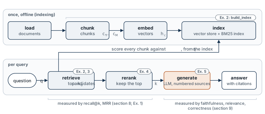
A RAG pipeline in two lanes. Offline, documents are loaded, chunked, embedded and indexed. Per query, the question retrieves candidates from the index, a reranker keeps the best k, and a language model generates an answer from them with citations. Retrieval is measured by recall at k and MRR, the answers by faithfulness, relevance and correctness. — Figure 1: The seven stages of the table below. Load, chunk, embed and index run once, offline; retrieve, rerank and generate run for every question, and retrieval embeds the question with the same encoder. Retrieval and generation are measured separately (sections 8 and 9), and the tags name the lab exercise that works on each stage.

Stage	When	What it does	In the lab
Load	once	read documents and their metadata	the committed snapshot of module pages 1–12 and the reading list
Chunk	once	cut each document into passages of about L tokens	`SentenceSplitter` (LlamaIndex)
Embed	once per chunk, once per query	map each chunk to a vector \mathbf{h}_c	a small open sentence encoder
Index	once	store the vectors (and, for BM25, the term counts) for fast search	`VectorStoreIndex`; `InMemoryVectorStore` (LangChain)
Retrieve	per query	score every chunk against q and keep the top k_0	Exercises 2 and 3
Rerank	per query	rescore the k_0 candidates with a slower, better scorer and keep the top k	Exercise 4
Generate	per query	prompt a language model with q and the k passages	Exercise 5

Every stage has settings, and every setting changes what the generator sees. The module’s second objective is to choose them from measurements, which needs a labeled question set (section 8). Without one, a RAG pipeline is tuned by looking at a few answers, which is how most of the failures in section 10 go unnoticed.

Check yourself. You change the chunk size from 256 to 128 tokens. Which of the seven stages must run again before the next query can be answered? And why do the gold evidence labels of section 8 not need to be redone?

Answer

Chunk, embed and index must run again: the chunks are different texts, so their vectors and the index built from them are stale. Load does not, because the documents have not changed. Retrieve, rerank and generate run per query in any case, now over the new chunks. The labels survive because they are spans of the source text, located by character offsets, and not chunk IDs. Whether a chunk covers a span is recomputed for any chunking. Labels tied to chunk IDs would have to be rewritten for every setting in a sweep.

3. Chunking

In this section: say what chunk size and overlap trade off, and name three ways chunking fails silently.

A retriever ranks chunks, not documents, and the generator reads only the chunks it is given. The chunk is the unit of evidence.

Small chunks (say L = 128 tokens) make each vector about one thing, so a precise question can match it. But the answer may be split across two chunks, and each chunk carries less context about what it is discussing.
Large chunks (L = 512 or more) keep explanations whole, but one vector must summarize several ideas, and each retrieved chunk spends more of the generator’s context.
Overlap L_o repeats the end of each chunk at the start of the next, so a sentence near a boundary appears whole in at least one chunk, at the price of storing and embedding some text twice.

On the briefing corpus, LlamaIndex’s SentenceSplitter with L_o = L/8 gives 1,867 chunks at L = 128, 907 at L = 256 and 459 at L = 512 on the lab’s snapshot (measured with Lab 13’s code). The splitter counts tokens of cl100k_base, the tokenizer bundled with LlamaIndex, not the embedding model’s own; and metadata that is embedded with a chunk also shrinks its effective size, which is one reason the lab excludes it.

The fair comparison between chunk sizes is at a fixed context budget, not at a fixed k. Passing k chunks of L tokens costs about

n_{\text{ctx}} = k\, L \tag{1}

input tokens per query, before the prompt and the question. Five chunks of 512 tokens and twenty of 128 cost the same; five of each do not. Section 8 measures recall against n_{\text{ctx}}.

Three ways chunking fails without an error:

Units differ between libraries. LlamaIndex’s SentenceSplitter(chunk_size=256) counts tokens of a tokenizer; LangChain’s RecursiveCharacterTextSplitter(chunk_size=256) counts characters by default. The same number gives chunks about four times apart in size.
The encoder truncates. Every encoder has a maximum input length, and text beyond it is dropped without a warning. The encoder the lab proposes accepts 512 tokens (model card, not checked on the Hub; the Hub was unreachable from the build environment); some popular small encoders accept 256 or fewer. A chunk longer than that is embedded from its beginning only.
Metadata is embedded too. By default LlamaIndex prepends each node’s metadata to the text it embeds (slug: 01-text-as-data followed by the chunk), and its BM25 retriever indexes the same text. That can help (a title is informative) or hurt (a file name is not), but it means two frameworks given the same chunks and the same encoder rank them differently. We measured this: with the metadata embedded, LlamaIndex and LangChain agreed on the top 5 for 3 of 6 test queries; with it excluded, on 6 of 6, with identical scores (build environment, stand-in encoder, 2026-10-05). The lab’s Exercise 3 turns on it.

Check yourself. Suppose a sweep reports recall@5 of 0.80 with L = 512 and 0.62 with L = 128 (invented numbers). A colleague concludes that 512-token chunks retrieve better. What is unfair about the comparison, and which run would make it fair? Separately: the colleague’s LangChain splitter was set to chunk_size=128. What chunk size did it really use?

Answer

By Equation 1, five chunks of 512 tokens put n_{\text{ctx}} = 2{,}560 tokens in front of the generator, and five of 128 put 640. The larger chunks were given four times the text, so they had four times the chance to contain the evidence. The fair comparison holds n_{\text{ctx}} fixed: L = 512 at k = 5 against L = 128 at k = 20. On the second question: that splitter counts characters by default, so its chunks were 128 characters, roughly a quarter of 128 tokens. The number in the configuration is not the chunk size until you know its unit.

4. Dense Retrieval

In this section: say how a bi-encoder scores a chunk, why its vectors can be computed ahead of time, and how it is trained.

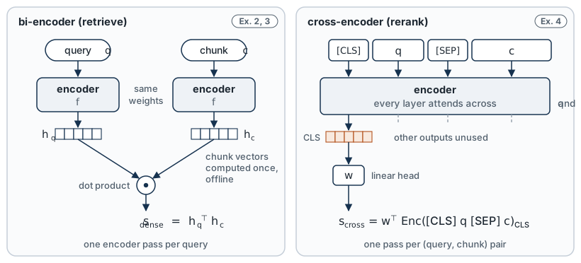
A dense retriever encodes the query and each chunk separately into unit vectors in \mathbb{R}^{d} and scores them by their dot product, which for unit vectors is Module 2’s cosine:

s_{\text{dense}}(q, c) = \mathbf{h}_q^\top \mathbf{h}_c, \qquad \mathbf{h}_x = \frac{f(x)}{\lVert f(x) \rVert} . \tag{2}

The encoder f is a transformer encoder (Module 6) whose token vectors are pooled into one vector, for example by averaging or by taking the first token’s vector. Because query and chunk never meet inside the network, this architecture is called a bi-encoder, and its key property follows: the M chunk vectors are computed once, at indexing time. A query then costs one encoder pass plus M dot products, and retrieval returns

R_k(q) = \operatorname*{top\text{-}k}_{c \in \mathcal{C}}\; s(q, c) , \tag{3}

the k chunks with the highest scores, in order. For 907 chunks and d = 384 that is about 350,000 multiply-adds per query, which is nothing; the lab searches exhaustively. Collections of millions of chunks use approximate nearest-neighbor indexes, which trade a little recall for speed (optional callout below).

How such an encoder is trained. Word vectors (Module 2) were learned by telling real (word, context) pairs from random ones. Sentence encoders for retrieval are trained the same way, with (query, relevant passage) pairs in place of (word, context) pairs. For a query q with a relevant passage c^+ and a batch of B passages c_1, \dots, c_B that contains c^+, the contrastive loss with in-batch negatives (Karpukhin et al., 2020) is a softmax cross-entropy over the batch:

\mathcal{L}_{\text{con}}(q) = -\log \frac{\exp\big(s_{\text{dense}}(q, c^+) / \tau\big)}{\sum_{j=1}^{B} \exp\big(s_{\text{dense}}(q, c_j) / \tau\big)} . \tag{4}

The other passages in the batch, relevant to other queries, serve as negatives for free. Compare Module 2’s negative-sampling loss: it scored each negative with a separate sigmoid; here the negatives compete with the positive in one softmax, as in Module 1’s cross-entropy with the passages as classes. The temperature \tau (typically 0.01 to 0.05) sharpens the softmax, as Module 11’s temperature does with logits.

Worked example: one query, three chunks. Take d = 2 and unit vectors \mathbf{h}_q = (0.6, 0.8), \mathbf{h}_{c_1} = (1, 0), \mathbf{h}_{c_2} = (0, 1) and \mathbf{h}_{c_3} = (0.8, 0.6).

Scores (Equation 2): s_{\text{dense}}(q, c_1) = 0.60, s_{\text{dense}}(q, c_2) = 0.80 and s_{\text{dense}}(q, c_3) = 0.48 + 0.48 = 0.96.
Top-2 list (Equation 3): R_2(q) = (c_3, c_2).
Training loss (Equation 4), with the three chunks as the batch and c_3 as the relevant passage c^+. At \tau = 0.05 the scores become the logits 12, 16 and 19.2, and \mathcal{L}_{\text{con}} = -\log \dfrac{e^{19.2}}{e^{12} + e^{16} + e^{19.2}} = 0.041. At \tau = 1 the logits are the scores themselves, and the loss is 0.936.

The ranking is the same at both temperatures. What changes is how much of the softmax’s probability the positive receives: a margin of 0.16 in cosine is a margin of 3.2 in the logits at \tau = 0.05. Cosines live in [-1, 1], so without a small \tau the loss could never get close to zero, however well the encoder ranked.

What the loss implies for use: the encoder knows the kinds of similarity its training pairs taught it. A model trained on web questions and answers matches paraphrases well (“why is attention scaled?” finds “the dot products grow with the dimension”) and may match an exact identifier, a number or a rare symbol poorly. That is what sparse retrieval is good at.

Check yourself. In the worked example, suppose the relevant passage is c_1 and not c_3. What is the contrastive loss at \tau = 0.05? In which direction does a gradient step move \mathbf{h}_q? And which of the four vectors would have to be recomputed at query time for a new question?

Answer

The logits are still 12, 16 and 19.2, but the positive is now the smallest: \mathcal{L}_{\text{con}} = -\log \dfrac{e^{12}}{e^{12} + e^{16} + e^{19.2}} = 7.24, about 180 times the loss when c_3 was the positive. Minimizing it raises s_{\text{dense}}(q, c_1) and lowers the scores of the in-batch negatives, most strongly c_3, which holds nearly all the softmax’s probability. The encoder’s weights move so that \mathbf{h}_q turns toward \mathbf{h}_{c_1} and away from \mathbf{h}_{c_3}. At query time only \mathbf{h}_q is computed. The three chunk vectors were stored at indexing time, which is the property that makes a bi-encoder fast.

In the lab. In Exercise 2 you write build_index(docs, chunk_size, overlap, embed_model): a SentenceSplitter with deterministic node IDs and the metadata excluded from embedding, then a VectorStoreIndex, whose retriever computes Equation 2 and Equation 3. A provided cell sweeps L \in \{128, 256, 512\} and k from 1 to 10 on the dev questions and plots recall against n_{\text{ctx}} (Equation 1). Equation 4 is not implemented: the encoder comes pretrained with a loss of this family (see its model card).

Optional: Approximate Nearest-Neighbor Search

Exhaustive search over M vectors costs O(Md) per query. Above about a million chunks, vector databases use approximate indexes instead: a graph over the vectors in which a greedy walk reaches near neighbors in roughly logarithmic time (HNSW), or a coarse clustering in which only the closest clusters are searched (IVF), often with compressed vectors. They return most, not all, of the true top k. The fraction they return is itself a recall, measured against exhaustive search, and it is separate from the retrieval recall of section 8: an index can be perfect at finding the nearest vectors and the nearest vectors can still be the wrong passages.

5. Sparse and Hybrid Retrieval

In this section: say when BM25 beats a dense retriever, and combine the two rankings.

Sparse retrieval scores a chunk by the query words it contains. Module 1’s optional section derived BM25. With \mathrm{tf}(w, c) the count of word w in chunk c, |c| the chunk’s length in tokens, \mathrm{avgdl} the mean length and \mathrm{df}(w) the number of chunks that contain w:

s_{\text{BM25}}(q, c) = \sum_{w \in q} \mathrm{idf}(w)\cdot \frac{\mathrm{tf}(w, c)\,(k_1 + 1)}{\mathrm{tf}(w, c) + k_1\bigl(1 - b + b\,\frac{|c|}{\mathrm{avgdl}}\bigr)}, \qquad \mathrm{idf}(w) = \log\Bigl(\frac{M - \mathrm{df}(w) + 0.5}{\mathrm{df}(w) + 0.5} + 1\Bigr). \tag{5}

The vector of a chunk is as long as the vocabulary and mostly zeros, hence “sparse”. BM25 needs no training, and it finds exactly what a dense encoder may blur: an equation label, a model ID such as Qwen2.5-0.5B-Instruct, a number such as 0.8669. It fails on paraphrase: a question that uses none of the passage’s words scores zero. On a benchmark of 18 retrieval datasets, Thakur et al. (2021) found BM25 a strong baseline that many dense retrievers failed to beat outside the domain they were trained on.

The library the lab uses for BM25, llama-index-retrievers-bm25 0.8.0, computes Equation 5 without the factor (k_1 + 1) in the numerator, as Lucene does. That scales every score by the same constant and leaves the ranking unchanged. We checked it against Module 1’s formula on a small corpus: equal to within about 10^{-6} after dividing by k_1 + 1 (float32 arithmetic in the library), with k_1 = 1.5 and b = 0.75 (build environment, 2026-10-05). It also removes English stopwords and, by default, stems words.

Hybrid retrieval combines the two. Their scores are on different scales (cosines between -1 and 1, BM25 sums without an upper bound), so adding them needs a normalization and a weight, both of which must be tuned. Reciprocal rank fusion (Cormack et al., 2009) uses ranks instead of scores:

s_{\text{RRF}}(q, c) = \sum_{r \in \{\text{dense},\, \text{BM25}\}} \frac{1}{r_0 + \mathrm{rank}_r(c \mid q)}, \qquad r_0 = 60 , \tag{6}

where a chunk missing from a ranker’s list contributes nothing for that ranker. The constant r_0 damps the advantage of the very top ranks; Cormack et al. fixed it at 60 in a pilot and did not tune it further. Worked example: a chunk ranked 1st by the dense retriever and 10th by BM25 scores 1/61 + 1/70 = 0.0307; a chunk ranked 3rd by both scores 2/63 = 0.0317 and comes first. RRF rewards agreement.

Check yourself. Chunk A is ranked 1st by the dense retriever and does not appear in BM25’s list. Chunk B is ranked 5th by both. Which has the higher RRF score (Equation 6, r_0 = 60)? How far down both lists could B sit and still beat A?

Answer

A scores 1/61 = 0.0164, with nothing from BM25. B scores 2/65 = 0.0308, nearly twice as much. In general a chunk at rank r in both lists beats A when 2/(60 + r) > 1/61, that is when r < 62: even 61st place in both lists (2/121 = 0.0165) edges out a single first place. With r_0 = 60, RRF values agreement between the rankers far above one ranker’s enthusiasm. That is a design choice to know about: a chunk that only the dense retriever can find, such as a pure paraphrase, is pushed down by hybrid fusion.

In the lab. The stretch section builds BM25 with BM25Retriever over the same chunks (metadata excluded, stemming off for the check), confirms that its scores equal Lab 1’s bm25_scores divided by k_1 + 1 (Equation 5), and asks you to write rrf(rankings, r0=60) (Equation 6). You then compare dense, BM25 and hybrid recall@k on test, broken down by question kind. LlamaIndex has a fusion retriever too, but it calls a language model by default even when it does not need one (section 11).

6. Reranking: Cross-Encoders and a Decision Model

In this section: say why a reranker scores better than the first-stage retriever, what it costs, and how a decision model can serve as one.

A bi-encoder compresses each chunk into one vector before it has seen the query. A cross-encoder reads the query and the chunk together, as one input, so every layer of attention can compare them word by word:

s_{\text{cross}}(q, c) = \mathbf{w}^\top \mathrm{Enc}\big([\texttt{CLS}]\; q\; [\texttt{SEP}]\; c\big)_{\texttt{CLS}} , \tag{7}

where \mathrm{Enc}(\cdot)_{\texttt{CLS}} is the encoder’s output vector at the first position and \mathbf{w} a learned vector. This is Module 6’s classification head on a sentence pair, trained to tell relevant pairs from irrelevant ones (Nogueira and Cho, 2019, did this with BERT on a passage-ranking dataset). It is usually more accurate than Equation 2, but nothing can be precomputed: scoring all 905 chunks would take 905 encoder passes per query.

Hence two stages. Retrieve k_0 candidates cheaply (say 20) with the bi-encoder, BM25 or both; rescore only those with the cross-encoder; keep the top k. The reranker cannot recover a chunk the first stage missed, so k_0 is chosen by the first stage’s recall@k_0 (section 8), and k by the generator’s budget (Equation 1). The cost is k_0 pair evaluations per query.

A bi-encoder encodes the query and the chunk separately with shared weights and compares their vectors with a dot product; a cross-encoder reads the query and the chunk together as one input and a linear head on its first output gives one relevance score. — Figure 2: Left, a bi-encoder (Equation 2): the query and the chunk are encoded separately by the same encoder, so every chunk vector can be computed once, offline, and a query costs one encoder pass. Right, a cross-encoder (Equation 7): the query and the chunk are read together, so attention can compare them word by word, at the price of one encoder pass per (query, chunk) pair. That price is why the cross-encoder only reranks the k_0 candidates the bi-encoder retrieved.

A decision model as a reranker. Reranking is a typed judgment repeated many times: for this question, how relevant is this passage? That is the shape of question Module 12’s decision model answers. Jev’s Score question places a state on an ordered rubric and returns a probability \pi(\ell \mid q, c) for each level \ell and a score field that typesafe-sdk 0.7.2 describes as the probability-weighted average of the levels. With a four-level rubric (0: off-topic; 1: related but without the answer; 2: part of the answer; 3: the full answer), we rank by that expected level:

\bar{\ell}(q, c) = \sum_{\ell=0}^{3} \ell\; \pi(\ell \mid q, c) . \tag{8}

Everything in that sentence is the interface: one system_one(state, questions) call per (query, passage) pair, with state {"question": q, "passage": c} and one Score question, and the score field read back. Four points from Module 12 carry over.

There is no official LlamaIndex integration. No package from TypeSafe or from LlamaIndex connects them (checked 2026-10-05). The lab writes the reranker itself, in about 35 lines, as a subclass of LlamaIndex’s BaseNodePostprocessor. Install only typesafe-sdk; other packages with similar names are not TypeSafe’s.
There is no batch endpoint. k_0 candidates mean k_0 calls, sent concurrently with AsyncTypeSafeClient under a limit (the lab uses 8).
Rank by the probabilities, not confidence. Equation 8 uses \pi; the confidence field measures how concentrated \pi is (Module 12, section 8). The lab stores it beside each passage and does not sort by it.
Fail open. If a call fails, the reranker returns the first stage’s order unchanged and says so. A reranker that fails closed would turn a network error into an empty context.

We do not know how Jev was trained or how it represents a passage. TypeSafe states that its models are “trained for calibrated decisions; validate their performance in the target domain” (Module 12, section 5). Whether its relevance judgments help on our corpus is what the lab’s labeled questions measure, against a cross-encoder, on the same candidates. Nothing about Jev’s ranking quality is assumed on this page.

Check yourself. (1) A first stage has recall@5 of 0.60 and recall@20 of 0.85 (invented numbers). You rerank its 20 candidates and keep 5. What is the highest recall@5 the reranker can reach, and how many pair evaluations do 80 questions cost? (2) For one query, passage X gets rubric probabilities \pi = (0.1, 0.2, 0.3, 0.4) over levels 0 to 3, and passage Y gets (0.45, 0, 0, 0.55). Which ranks first under Equation 8? Which has the higher probability of being a full answer?

Answer

At most 0.85. A reranker reorders the k_0 = 20 candidates and cannot add a chunk that the first stage missed, so its ceiling is the first stage’s recall@20. The cost is 80 \times 20 = 1{,}600 pair evaluations. (2) \bar{\ell}(X) = 0.2 + 0.6 + 1.2 = 2.0 and \bar{\ell}(Y) = 3 \times 0.55 = 1.65, so X ranks first, although Y is more likely to be a full answer (0.55 against 0.40). The expected level counts Y’s 0.45 chance of being off-topic against it. Y’s distribution is also the more concentrated of the two, which is one more reason not to sort by a number that measures concentration.

In the lab. In Exercise 4 you write relevance_question(query), which returns the Score question with the four-level rubric, and rerank_by_scores(nodes, scores, top_n), which sorts candidates by a score, keeps the first stage’s order among ties, and keeps the top n. Two provided postprocessors call them: JevRerank (with a TYPESAFE_API_KEY; Equation 8) and CrossEncoderRerank (otherwise; Equation 7). Checkpoints run on a fake client that returns real typesafe_sdk response objects, including a failure that must fall back to retrieval order. A provided cell prints recall@k and MRR before and after reranking, latency per query and, with a key, the measured Jev tokens and cost.

7. Generation: Sources, Citations, Abstention

In this section: write a generation prompt whose output can be checked.

The generator is Module 8’s provider wrapper, with a prompt that does three things:

Numbers the sources. Each passage appears as [1] (03-sequence-models › 2. Vanishing gradients) ..., in rank order, best first (section 1: the middle of a long context is used worst).
Asks for citations. Each sentence of the answer ends with the numbers of the sources it uses. Citations make section 9’s checks possible and let a reader verify the answer.
Defines abstention exactly. If the sources do not contain the answer, the model must reply with one fixed sentence, “I cannot answer from the provided sources.” A fixed string can be detected by a program; “I’m not sure, but…” cannot. Module 8’s rule applies: design the output so that a programmatic check exists.

The passages are data, not instructions. Retrieved text can contain instructions: Module 8’s section on prompt injection quotes one, so a question about prompt injection retrieves it. The prompt says that the sources are quotations to be used as evidence, which reduces the risk without removing it (Module 8, section 8). An attack that arrives through retrieved content rather than through the user is called indirect prompt injection (Greshake et al., 2023). Module 14 tests it on an agent with a tool that can act.

Check yourself. For a question whose answer is not in the sources, the generator replies: “I could not find this in the provided sources, but I believe the value is 0.9.” How does a program that follows this section’s contract classify the reply, and why is that the right design?

Answer

As an answer, not an abstention: it is not the fixed sentence. It is then an answer whose claim cites no source, and section 9’s faithfulness judge will find nothing in the passages to support “the value is 0.9”. That is the right outcome. The reply states a fact from the model’s parametric memory while sounding cautious, and a reader cannot check it. Had the contract accepted any hedged wording as an abstention, the program would need a model to decide which replies count, and the abstention rate would depend on that judge. A fixed string needs only a comparison.

8. Evaluating Retrieval

In this section: define recall@k and MRR against labeled evidence, and use them to choose settings.

Retrieval and generation fail in different ways, so the module’s third objective is to measure them separately. Retrieval is measured against gold evidence: for each answerable question q, people have marked the text that answers it. Two complications shape the definition.

Labels must not depend on the chunking, or a chunk-size sweep would need new labels for every setting. So the evidence is a span of the source text (a quoted sentence or two, located by character offsets), and a chunk covers a span when it contains at least half of it.
Some questions need more than one piece of evidence, and some pieces can be found in more than one place. So G(q) = \{g_1, \dots, g_m\} is a set of groups: every group is needed, and any one span in a group will do.

Recall@k is the fraction of a question’s evidence groups covered by its top k chunks, averaged over the N answerable questions:

\mathrm{Recall@}k = \frac{1}{N} \sum_{q} \frac{1}{|G(q)|} \sum_{g \in G(q)} \max_{c \in R_k(q)}\; \max_{e \in g}\; \mathrm{cov}(c, e), \tag{9}

where \mathrm{cov}(c, e) = 1 if chunk c covers span e and 0 otherwise. For a question with one group this is 1 if any of the top k chunks contains the evidence, which some papers call the hit rate or success@k.

Mean reciprocal rank asks how high the first useful chunk sits:

\mathrm{MRR} = \frac{1}{N} \sum_{q} \frac{1}{\mathrm{rank}_1(q)}, \tag{10}

where \mathrm{rank}_1(q) is the position of the first chunk that covers any span of any group, and the term is 0 if no chunk in the list does. Recall@k says whether the evidence reached the generator; MRR says whether it arrived near the top, which matters because the generator reads the top best (section 1).

Worked example: recall@5 and MRR on three questions. Question A has one group, covered first at rank 3. Question B needs two groups; within the top 5, only one is covered, at rank 1. Question C’s evidence is not in the top 10. Then Recall@5 = (1 + \tfrac12 + 0)/3 = 0.5 and MRR = (\tfrac13 + 1 + 0)/3 = 0.444.

Using the numbers to choose. Three rules, each from earlier modules.

Compare at equal cost. Plot recall against n_{\text{ctx}} (Equation 1), not against k.
Choose on dev, report on test. Chunk size, k and the reranker are hyperparameters. Choosing them on the same questions you report makes the report optimistic, as with Module 11’s temperature and Module 12’s thresholds.
Read differences with their noise. With N = 50 questions and a recall near 0.8, Module 8’s standard error is \sqrt{0.8 \times 0.2 / 50} \approx 0.06. Two settings measured on the same questions are better compared pairwise: count the questions one setting gets and the other misses, in both directions. Seven gained and two lost is suggestive but not significant (two-sided sign test, p \approx 0.18); eight and one would be (p \approx 0.04); four and three is noise.

Demo: equal k or equal budget? The toy data are invented for this demo and are not measurements from Lab 13: for 12 questions with one evidence group each, the rank at which the evidence is first covered, at three chunk sizes. The left panel plots recall@k (Equation 9) against k; the right panel plots the same curves against n_{\text{ctx}} = kL (Equation 1). Predict first. At k = 5 the 512-token chunks have the highest recall. Will they still be ahead when all three sizes get the same 2,560 tokens?

viewof budget13 = Inputs.range([512, 2560], {value: 2560, step: 128, label: "context budget n_ctx (tokens)"})

{
  // Rank of the first chunk that covers each question's evidence (Infinity: never retrieved). Invented.
  const ranks = {128: [1, 2, 3, 4, 5, 6, 8, 9, 12, 15, 18, Infinity], 256: [1, 1, 2, 3, 3, 4, 5, 6, 8, 10, 14, Infinity],
                 512: [1, 1, 2, 2, 3, 3, 4, 5, 7, 9, Infinity, Infinity]};
  const recall = (L, k) => ranks[L].filter(r => r <= k).length / ranks[L].length;    // eq-recall with one group each
  const sizes = [128, 256, 512], name = L => `L = ${L}`;
  const color = {domain: sizes.map(name), range: ["var(--demo-orange)", "var(--demo-grey)", "var(--demo-blue)"], legend: true};
  const curve = sizes.flatMap(L => Array.from({length: 20}, (_, i) => ({L: name(L), k: i + 1, n: (i + 1) * L, r: recall(L, i + 1)})));
  const at = sizes.map(L => { const k = Math.floor(budget13 / L); return {L: name(L), k, n: k * L, r: recall(L, k)}; });
  const panel = (x, label, domain, extra) => Plot.plot({width: 360, height: 320, grid: true, color,
    x: {label, domain}, y: {domain: [0, 1], label: "recall@k"},
    marks: [Plot.line(curve, {x, y: "r", stroke: "L", curve: "step-after", clip: true}), ...extra,
            Plot.dot(at, {x, y: "r", fill: "L", r: 5})]});
  const left = panel("k", "number of chunks k", [1, 20], []);
  const right = panel("n", "context tokens n_ctx = k · L", [0, 2700],
    [Plot.ruleX([budget13], {stroke: "currentColor", strokeDasharray: "2 3"})]);
  return html`<div style="display:flex;gap:1rem;flex-wrap:wrap">${left}${right}</div>
    <p><strong>Budget ${budget13} tokens</strong>: ${at.map(d => `${d.L} reads k = ${d.k} chunks, recall@k ${d.r.toFixed(2)}`).join("; ")}.</p>`;
}

What it shows. The dots mark what each chunk size retrieves within the budget, k = \lfloor n_{\text{ctx}} / L \rfloor chunks. In the left panel the dots sit at different k, and reading across at one k favors the large chunks: at k = 5, recall is 0.67 for L = 512 and 0.42 for L = 128. In the right panel the dots line up near the budget line, and the order is reversed: at 2,560 tokens, 0.67 for five 512-token chunks against 0.92 for twenty 128-token chunks. Nothing about the retriever changed between the panels, only the axis. Which chunk size wins at equal budget on a real corpus is an empirical question, and the sweep after Lab 13’s Exercise 2 is how you answer it.

Who labels. The questions and their evidence are written and checked by people, not generated by a model. A model asked to write questions from a passage tends to reuse the passage’s words, which flatters BM25 and any encoder that matches surface form, and a model that judges relevance is the kind of judge section 9 asks you to check, not to trust. The lab’s question set follows the rule of the Module 11 decision set: no item written or labeled by a language model.

Check yourself. Question D needs two evidence groups: g_1 = \{e_1, e_2\} (either span will do) and g_2 = \{e_3\}. Its ranked list covers nothing at rank 1, e_2 at rank 2, e_1 at rank 3, nothing at rank 4 and e_3 at rank 5. Compute D’s recall@3, recall@5 and reciprocal rank. Then add D to the worked example’s three questions and recompute Recall@5 and MRR over all four.

Answer

At k = 3 only g_1 is covered, so D’s recall@3 is 1/2. The spans e_1 and e_2 are alternatives within one group: finding both does not count twice. At k = 5 both groups are covered, so recall@5 is 1. The first chunk that covers any span is at rank 2, so the reciprocal rank is 1/2. Over the four questions, Recall@5 = (1 + \tfrac12 + 0 + 1)/4 = 0.625 and MRR = (\tfrac13 + 1 + 0 + \tfrac12)/4 = 0.458. D illustrates why both metrics are reported. Its reciprocal rank is good, and yet a generator given only the top 3 would see half the evidence.

In the lab. In Exercise 1 you write recall_at_k(ranked, groups, k) (Equation 9) and reciprocal_rank(ranked, groups) (one term of Equation 10), with covers provided. Checkpoint: the worked example above, plus edge cases (a question with no gold groups raises an error; a span split exactly in half by a chunk boundary counts as covered). Exercises 2, 3 and 4 then report both metrics, on dev to choose and on test to report, with N and the pairwise gained/lost counts.

9. Evaluating Answers

In this section: define faithfulness, answer relevance and correctness, and say what each misses.

Once the passages are fixed, the answer can still go wrong in two independent ways: it can say things the passages do not support, and it can fail to answer the question. Three measures, all per answered question.

Faithfulness. Split the answer into sentences a_1, \dots, a_n (we treat a sentence as one claim; a sentence can hold several, which is a simplification), drop the citations, and ask a judge whether each is supported by the retrieved passages R:

\mathrm{Faith} = \frac{1}{n} \sum_{j=1}^{n} \mathbf{1}\big[J(a_j, R) \ge \tfrac12\big] . \tag{11}

An abstention has no claims; it is counted separately, not as faithful.

Answer relevance. Does the answer address the question that was asked? A faithful answer can quote the passages accurately and still answer a different question. RAGAS (Es et al., 2024) measures it by generating questions from the answer and comparing them with the original by embedding similarity; the lab uses a three-level judged rubric (answers it, partly, not at all) instead, and prints it without building anything on it.

Correctness. Is the answer right? For questions whose answer is a short fact (a number, a name, a symbol), people record the acceptable forms when they write the question, and a program checks whether the answer contains one. That is preferred whenever it is possible (Module 8). Correctness is not faithfulness: a faithful answer to a wrong passage is wrong, and an unfaithful answer from the model’s parametric memory can be right.

Unanswerable questions. Some questions in the set have no answer in the corpus. The right output is the abstention sentence. Report the abstention rate on those and the false-abstention rate on answerable ones; Module 15 turns the pair into a cost.

Separating the two failures. For each answerable question, cross whether retrieval covered its evidence with whether the answer was correct:

	answer correct	answer wrong or abstained
evidence retrieved	the pipeline worked	a generation failure: fix the prompt or the model
evidence not retrieved	answered from parametric memory, or luck: not grounded	a retrieval failure: fix chunking, k, the retriever or the reranker

The table tells you which half of the pipeline to work on. It is the reason the module measures retrieval and answers separately.

The judge is a model, and Module 8’s caveats apply to it. It can be wrong, swayed by length and fluency, and its verdicts change with its prompt and version. Three more for this use:

A model grading its own output may be lenient with it. When you have keys for two providers, let one generate and the other judge.
A natural-language-inference (NLI) model (a cross-encoder trained to label a premise and a hypothesis as entailment, contradiction or neutral) is the lab’s open judge: J is the largest entailment probability of the sentence over the passages. It is small and deterministic, but it was trained on short everyday sentences, and module pages full of notation and equations are far from that.
Faithfulness is only as good as its agreement with people. Before trusting a judge, compare its verdicts with human labels on a sample and report the agreement (Module 8). Until the lab’s audit set exists, its faithfulness numbers are printed as unvalidated.

Check yourself. An answer has four sentences, and the judge gives them support probabilities 0.9, 0.55, 0.4 and 0.8. (1) What is its faithfulness (Equation 11)? (2) The 0.4 sentence states a fact that is true but appears in none of the retrieved passages, and it is the sentence that answers the question; the question’s gold evidence was not retrieved. In which cell of the two-by-two table does this question fall, and is it a success?

Answer

Three of the four sentences reach the threshold of \tfrac12, so \mathrm{Faith} = 3/4 = 0.75. (2) The answer is correct and the evidence was not retrieved: the lower-left cell, “answered from parametric memory, or luck: not grounded”. It is not a success of the pipeline. Retrieval failed on this question, and the correct sentence is the unfaithful one, so a reader cannot check it against a source. Correctness alone would have scored the question as a win and hidden a retrieval failure. Faithfulness alone would have flagged the one sentence that was right. This is why the two are measured separately and then crossed.

In the lab. In Exercise 5 you write faithfulness(answer, sources, judge, threshold=0.5) (Equation 11), returning the score and the per-sentence verdicts, with None for an abstention. Checkpoint: a fake judge with known verdicts, citations stripped before judging, abstention handled. A provided cell generates answers for the test questions through the PROVIDER switch, scores faithfulness with the selected judge, checks correctness against the recorded answer forms, prints abstention on unanswerable questions, and fills the two-by-two table above. No answer metric is asserted.

10. Common Failures

In this section: name the usual failures and the measurement that reveals each.

Failure	Symptom	Revealed by
The answer is not in the corpus	a confident wrong answer instead of an abstention	unanswerable questions in the evaluation set
Evidence ranked just below k	right answer at k = 10, wrong at k = 5	recall@k as a curve in k; a reranker
Evidence split by a chunk boundary	each half retrieved alone looks irrelevant	recall by chunk size; overlap
Encoder truncation	long chunks never match their second half	recall falling as L grows past the encoder’s limit
Vocabulary mismatch	a paraphrased question misses with BM25	dense against BM25, by question kind
Exact identifiers missed	a number or model ID misses with a dense encoder	the same comparison; hybrid retrieval
The generator ignores the context	the answer contradicts a retrieved passage	faithfulness; the two-by-two table
Evidence in the middle of a long context	right passage retrieved, answer still wrong	MRR; fewer, better-ranked passages
Instructions inside retrieved text	the answer follows the passage, not the user	an injection item (Module 14)
A stale index	answers about a page as it used to be	a version or date in each chunk’s metadata
Questions written from the chunks	high recall that does not survive real questions	a human-written question set with paraphrase

Check yourself. Your pipeline answers correctly with k = 10 and wrongly with k = 5 on many questions, and its MRR is low. A teammate proposes to ship with k = 10. Name the failure, give one cost of the proposal, and name the alternative that this module would have you measure against it.

Answer

The failure is “evidence ranked just below k”: the first stage finds the evidence but ranks it low, which is what a low MRR says. Shipping k = 10 doubles n_{\text{ctx}} (Equation 1) and with it the input cost of every query, and it places the useful passage in the middle of a longer context, where models use it worst. The alternative is a reranker over the same candidates: keep k_0 = 10 or 20 for retrieval, rerank, and pass k = 5. Measure both on dev, record the context tokens each uses, and count the questions each gains and loses before choosing.

11. LlamaIndex and LangChain

In this section: say what each framework abstracts, where they overlap, and which interfaces the lab uses.

Both frameworks wrap the same stages; they start from different ends.

	LlamaIndex	LangChain
Centered on	data: documents to an index to a query	composition: small parts joined into chains
Document and chunk	`Document`, `TextNode` (with character offsets into the document)	`Document` (`page_content`, `metadata`)
Chunking	`SentenceSplitter` (tokens)	`RecursiveCharacterTextSplitter` (characters by default), in `langchain-text-splitters`
Encoder interface	`BaseEmbedding`	`Embeddings`
Index and search	`VectorStoreIndex`, `.as_retriever(similarity_top_k=k)`	`InMemoryVectorStore`, `.as_retriever(search_kwargs={"k": k})`
Reranking hook	`BaseNodePostprocessor`	none in the core; a function in the chain
Generation	query engines and response synthesizers with built-in prompts	prompt templates and chat models joined into a chain with the pipe operator
Control flow	workflows	LangGraph (Module 14)

Where they overlap. Almost everything up to retrieval: each has a document type, splitters, an encoder interface, vector stores and a retriever. They interoperate: a LangChain retriever is a Runnable, so any Python function, including a LlamaIndex retriever, can become one. The lab builds the same retriever in both and checks that they return the same chunks.

What they hide, and why the lab looks. Three defaults met in this module, all read in the installed source:

LlamaIndex embeds metadata with the text (section 3).
LlamaIndex gives every node a random ID unless you pass an ID function, so node IDs change from run to run. The lab passes one, so citations and labels are reproducible.
When no language model is configured, LlamaIndex components that may need one (query engines, the fusion retriever) try to load OpenAI’s and fail without the llama-index-llms-openai package or a key. The lab sets a mock model and does generation itself. LlamaIndex’s default question-answering prompt is short (“Context information is below. … Given the context information and not prior knowledge, answer the query.”); it asks neither for citations nor for an exact abstention sentence, which is why the lab writes its own.

The interfaces the lab subclasses or calls are few: BaseEmbedding (three methods), BaseNodePostprocessor (one), LangChain’s Embeddings (two) and BaseRetriever (one). Learn those, and a version change is a renaming exercise.

In the lab. In Exercise 3 you write make_lc_retriever(nodes, embed_fn, k): an InMemoryVectorStore over the same chunks and the same encoder, returned as a retriever, and a small chain that turns its output into the same passage records as Exercise 2. Checkpoint: for every dev question, the two frameworks return the same chunk IDs in the same order (ties aside), and the chain answers .invoke and .batch. A provided cell first shows what happens with LlamaIndex’s default metadata embedding.

Equations and Where You Implement Them

Equation	Lab 13
The original RAG model (optional callout)	not implemented
Context budget (Equation 1)	provided sweep after Exercise 2: recall plotted against n_{\text{ctx}}
Dense score and top-k (Equation 2, Equation 3)	Exercise 2: `build_index`, through `VectorStoreIndex`; Exercise 3: `make_lc_retriever`
Contrastive loss (Equation 4)	not implemented: the encoder is pretrained
BM25 (Equation 5)	Stretch: `BM25Retriever`, checked against Lab 1’s `bm25_scores`
Reciprocal rank fusion (Equation 6)	Stretch: `rrf`
Cross-encoder score (Equation 7)	provided `CrossEncoderRerank`, through `rerank_by_scores` (Exercise 4)
Expected rubric level (Equation 8)	provided `JevRerank` with `relevance_question` (Exercise 4); keyed path only
Recall@k and MRR (Equation 9, Equation 10)	Exercise 1: `recall_at_k`, `reciprocal_rank`; used in Exercises 2–4 and the stretch
Faithfulness (Equation 11)	Exercise 5: `faithfulness`

Summary

Retrieval gives a language model a non-parametric memory: text that is current, citable and far cheaper to send than a whole corpus. Long contexts do not replace it; models use the middle of a long context poorly.
A RAG pipeline has seven stages: load, chunk, embed and index once; retrieve, rerank and generate per query. Each has settings, and each setting should be chosen from measurements.
Chunk size trades precision against context; compare sizes at a fixed context budget (Equation 1). Libraries count chunk size in different units, encoders truncate, and LlamaIndex embeds metadata by default.
A bi-encoder scores by a dot product of precomputed vectors (Equation 2), trained with a contrastive loss (Equation 4) that generalizes Module 2’s negative sampling. BM25 (Equation 5) catches exact words that a dense encoder blurs; reciprocal rank fusion (Equation 6) combines the two by rank.
A cross-encoder (Equation 7) reads the query and the passage together: better, and too slow for the whole collection, so it reranks a few candidates. A decision model’s Score answer can rerank too, by the expected level of its probabilities (Equation 8), through a postprocessor we write, since no official integration exists. Whether it helps is measured, not assumed.
Retrieval is measured with recall@k (Equation 9) and MRR (Equation 10) against human-labeled evidence spans; answers with faithfulness (Equation 11), relevance, correctness and abstention. The two-by-two table says which half of the pipeline failed.
A judge is a model and must be checked against people; prefer a programmatic check of correctness wherever the answer allows one.

Gotchas and Troubleshooting

“A long context window makes retrieval unnecessary.” It costs every token on every call, and models use information in the middle of a long context less well (Liu et al., 2024).
“The best chunk size is the one with the highest recall@5.” Larger chunks reach higher recall at a fixed k because they contain more text. Compare at a fixed context budget.
“Dense retrieval is always better than BM25.” It is better at paraphrase and often worse at exact identifiers and numbers, and outside its training domain BM25 is a strong baseline.
“Same chunks plus same encoder means same results in any framework.” Not if one framework embeds metadata with the text, or counts chunk size in other units.
“The reranker can fix poor retrieval.” It can only reorder the k_0 candidates it is given.
“A faithful answer is a correct answer.” It is faithful to the retrieved passages, which may be the wrong ones.
“An LLM judge’s faithfulness score is a measurement.” It is a model’s opinion until its agreement with human labels has been measured.
“Jev’s confidence is the right number to rank passages by.” It measures how concentrated the distribution is. Rank by the expected level of the probabilities.
“Questions generated from the documents are a fine evaluation set.” They copy the documents’ wording and inflate recall, especially for BM25.

Next Steps

You can now build a retriever, measure it and choose its settings, and evaluate answers separately from retrieval. Module 14 gives an agent this retriever as one of its tools, beside a calculator and a mock email action, and puts Module 12’s router and guard into the graph. The retrieved text becomes part of the state the guard reads, which is where indirect prompt injection meets a tool that can act. Module 15 evaluates the whole system on this module’s held-out questions.