Reinforcement and Preference Learning

Day 3 · Using and Aligning LLMs Module 9 120 minutes (55 briefing, 55 lab, 10 debrief) 11:30 briefing · 13:25 lab · 14:20 debrief

Text generation as a reinforcement-learning problem, the policy gradient, and reward models learned from comparisons.

Open the lab in Colab PyTorch Hugging Face

Duration: 120 minutes (55 briefing, 55 lab, 10 debrief)
Level: 300 · Advanced
Lab runtime: Google Colab, CPU runtime · about 10 minutes of compute
Accounts and cost: Google. Free
Without API keys: the lab always runs its real models

What You Will Build

In this module you will:

Frame text generation as a reinforcement-learning problem
Derive and implement the policy gradient
Train a reward model from pairwise preferences

New terms, in the glossary: policy gradient, Bradley–Terry model, reward model.

Before You Start

Module 8 · LLMs Through APIs and its lab, and the modules before it: this module measures its results against theirs.
A Google account. Colab’s default CPU runtime is enough.
No API keys: the lab runs its own models throughout.

Where we are. Day 2 trained models to make a given text more likely: pretraining, fine-tuning, instruction tuning. Module 8 ended on what that leaves out: nothing in a response says how good it is. This module answers one question: how do we train a model toward “better” when all we have is a score for a finished response, or only a person’s choice between two responses?

In the Lab

Open the lab in Colab

6 exercises in 2 parts. The notebook budgets 50 minutes for them; the lab slot is 55 minutes. Each exercise you write is a # TODO stub with a folded solution beneath it and a checkpoint that passes or fails; where people tend to stall, a folded hint sits above the stub.

Task	Briefing section	Time
Part A · The Policy Gradient on a Toy Task
Exercise 0 · Read the Toy Environment	2	3 min
Exercise 1 · Returns and the REINFORCE Loss	2, 3, 5 (Reference)	12 min
Exercise 2 · A Baseline, and the Variance It Removes	4	9 min
Part B · Learning a Reward From Comparisons
Exercise 3 · The Bradley–Terry Rater	7	8 min
Exercise 4 · The Reward-Model Loss, and Training	8	12 min
Exercise 5 · Normalize and Save the Reward Model	8	6 min

Challenge · Noisier Raters

Optional, for anyone who finishes the core path early: the notebook’s stretch section, after the last checkpoint.

When you are done. Runtime → Disconnect and delete runtime releases the machine; your keys stay in Colab Secrets for the next lab.

Agenda

Minutes	Section	In the room
0–4	1. No Label for “Better”	—
4–9	2. The Minimum Reinforcement Learning	—
9–20	3. The Policy Gradient and REINFORCE	Check yourself (2 min)
20–32	4. Baselines and Variance	Demo (4 min)
32–35	6. Why Comparisons Instead of Scores	Predict (1 min)
35–44	7. The Bradley–Terry Model	Check yourself (3 min)
44–55	8. Training a Reward Model	—
55	Total	45 minutes of exposition, 10 of activities

Checks, demos and predictions listed here are part of the live session and its minutes; the others on the page are for reading afterwards.

Read now · Sections 1–4 and 6–8, in the agenda above.

Use in the lab · Exercise 0: section 2; Exercise 1: sections 2, 3 and 5 (section 5: Reference; the exercise restates what it needs); Exercise 2: section 4; Exercise 3: section 7; Exercises 4 and 5: section 8.

Read later · Section 5, Generation as Sequential Decisions (Reference); the collapsed callouts marked Optional; Further Reading.

Notation for This Module

Notation. The workshop notation applies; several letters take a new meaning here, and Module 10 keeps them.

Symbol	Meaning
x	a prompt; y = (y_1, \dots, y_T) a response of length T, as source and target in Module 4. Here y is never a class label
y_{<t}	y_1, \dots, y_{t-1}
s_t, a_t	state and action at step t. For text, s_t = (x, y_{<t}) and a_t = y_t. This a_t is not the RNN pre-activation of Module 3
\pi_\theta(a \mid s)	the policy: a distribution over actions given the state, with parameters \theta. For text it is the language model, \pi_\theta = P_\theta
r_t, R(x, y)	reward at step t; reward of a complete response. r is not the LoRA rank of Module 7, and R is not Module 8’s limit on retries
G_t	the return from step t onward (the reward-to-go); G = G_1 is the return of the whole episode
J(\theta)	expected return, the quantity we maximize
b_t	a baseline subtracted from G_t (section 4). Not a bias: no bias vector appears in this module
N	number of sampled responses in one gradient estimate; y^{(i)} is the i-th
\mathcal{D}_x, \mathcal{D}_{\text{pref}}	the distribution of prompts; the dataset of preference triples
a \succ b	“a is preferred to b”
(x, y_w, y_l)	a preference triple: y_w was preferred to y_l. The subscripts mean winner and loser; they are not tokens
u	latent quality of an item in the Bradley–Terry model (section 7)
\tau_{\text{label}}	the label temperature of a noisy rater (section 7), a temperature in the sense of Module 3. \tau alone stays the sampling temperature, and never denotes a trajectory
g(y)	the lab’s gold score: the hidden rule that generates its preferences
r_\phi	the reward model, with parameters \phi
\sigma	the logistic sigmoid, \sigma(a) = 1 / (1 + e^{-a}), as in Modules 2 and 3

\beta is left free on purpose: Module 10 uses it for the KL coefficient. A value function, mentioned once below, is written v_\psi in lowercase, because V is the vocabulary.

1. No Label for “Better”

In this section: say what supervised fine-tuning cannot express, and what we need in its place.

Module 7 turned a pretrained language model into an instruction follower with supervised fine-tuning (SFT): maximize the likelihood of a reference response y given an instruction x, the masked loss of Module 7. Module 8 then evaluated such models, and ended on a gap: a response carries no signal of its own quality.

SFT has three blind spots, and all three come from the same place: its only training signal is “make this exact text more likely”.

It cannot rank. Given two acceptable responses to one prompt, one clearer than the other, SFT has no way to say “prefer the first”. There is one target, and every other text counts as equally wrong.
It imitates everything in the demonstration. Every token of the reference is scored the same, including its padding, its verbosity and its mistakes. A model trained on demonstrations is at best as good as the demonstrator.
It never sees its own outputs. Training uses teacher forcing (Module 3): the model is always conditioned on the reference prefix, never on text it wrote. What it does after its own mistakes is never trained.

What we would like instead is a number R(x, y), a reward, for any response y the model writes, and a training rule that makes high-reward responses more likely. Two problems stand in the way.

Sampling is not differentiable. The model produces y by sampling one token at a time. There is no gradient of R(x, y) with respect to the model’s parameters through that sampling step. Sections 2 to 5 solve this with the policy gradient.
Where does R come from? Sometimes a program can compute it: the exact match of Lab 4 is a reward for date normalization. For “helpful” or “clear” there is no program. People can, however, compare two responses reliably. Sections 6 to 8 turn comparisons into a learned reward function, the reward model.

Module 10 puts the two halves together: it optimizes a language model against a reward model.

2. The Minimum Reinforcement Learning

In this section: define policy, reward, episode and return, and map each onto text generation.

Reinforcement learning (RL) studies an agent that acts in an environment to collect reward. At each step t:

the agent is in a state s_t;
it draws an action from its policy, a_t \sim \pi_\theta(\cdot \mid s_t);
the environment returns a reward r_t \in \mathbb{R} and the next state s_{t+1}.

A run from the first state to a terminal state is an episode. The return from step t is the reward collected from then on, and the return of the episode is the total:

G_t = \sum_{t'=t}^{T} r_{t'}, \qquad G = G_1 = \sum_{t=1}^{T} r_t . \tag{1}

The goal is a policy with a high expected return, J(\theta) = \mathbb{E}_{\pi_\theta}[G], the expectation taken over everything random in an episode: the policy’s draws and the environment’s responses.

Nothing in this definition says the reward is differentiable, or even known as a formula. The agent only sees the numbers r_t. That is the point: RL optimizes an objective we can evaluate but cannot differentiate.

Text generation is an episode. Take a prompt x and a decoder-only language model (Module 5).

RL	Text generation
state s_t	the prompt and the tokens so far, (x, y_{<t})
action a_t	the next token y_t \in V
policy \pi_\theta(a_t \mid s_t)	the language model, P_\theta(y_t \mid x, y_{<t}) = \mathrm{softmax}(z_t)[y_t]
transition	append y_t to the text; deterministic
episode end	an end token, or the length limit T_{\max}
reward	a score of the response, usually given once at the end

The probability of a whole response is the product of the per-step probabilities, the chain rule of Module 1 and the conditional factorization of Module 4:

\pi_\theta(y \mid x) = \prod_{t=1}^{T} \pi_\theta(y_t \mid s_t), \qquad \log \pi_\theta(y \mid x) = \sum_{t=1}^{T} \log \pi_\theta(y_t \mid s_t), \qquad s_t = (x, y_{<t}). \tag{2}

So the language model you trained in Modules 5 to 7 already is a policy. What changes in this module is the training signal, not the model.

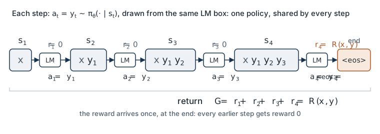
Text generation as a sequence of decisions: each state is the prompt plus the tokens so far, each action is the next token drawn from the language model, and the reward arrives at the end of the response. — Figure 1: Text generation as a sequence of decisions, drawn for a response of T = 4 tokens, the last one the end token. The state s_t = (x, y_{<t}) is the prompt and the tokens so far, and the action a_t = y_t is drawn from the same language model \pi_\theta at every step. With a reward for the whole response, r_t = 0 before the last step and r_T = R(x, y), so the return G of Equation 1 is R(x, y).

In the lab. The first half of Lab 9 uses a toy environment whose optimum you know. The policy writes T = 6 symbols from a vocabulary of 8, conditioned on its position and the previous symbol (a bigram policy, as in Module 1). The reward is the fraction of positions that match a hidden target string y^\star. The optimal policy writes y^\star with probability 1 and earns J = 1; the uniform policy, where training starts, earns J = 1/8. The provided token_logprobs(logits, actions) returns the per-step terms of Equation 2 for a batch, shape (N, T).

Check yourself. In the lab’s toy task (T = 6 symbols from a vocabulary of 8) the policy starts uniform. What is \log \pi_\theta(y \mid x) for any response y? With what probability does the policy write the target y^\star exactly? If the reward were 1 for an exact match and 0 otherwise, what would training see in a batch of 64 samples?

Answer

By Equation 2, \log \pi_\theta(y \mid x) = 6 \log \tfrac{1}{8} \approx -12.48 for every response. An exact match has probability (1/8)^6 = 1/262{,}144, about 3.8 \times 10^{-6}. With an all-or-nothing reward, almost every batch of 64 would contain only zeros, and a zero reward carries no information about which direction is better. The lab’s reward is the fraction of matching positions, which is 1/8 on average at the start and differs from sample to sample, so there is a signal to follow from the first step. How a reward is shaped decides whether the policy gradient has anything to work with.

3. The Policy Gradient and REINFORCE

In this section: derive the gradient of the expected reward, and turn it into a loss that autograd can use.

Let R(x, y) be the reward of a complete response (section 5 returns to per-step rewards). The objective is the expected reward of the model’s own samples, averaged over prompts:

J(\theta) = \mathbb{E}_{x \sim \mathcal{D}_x}\, \mathbb{E}_{y \sim \pi_\theta(\cdot \mid x)}\big[R(x, y)\big], \qquad \mathbb{E}_{y \sim \pi_\theta(\cdot \mid x)}\big[R(x, y)\big] = \sum_{y} \pi_\theta(y \mid x)\, R(x, y), \tag{3}

where the sum runs over all possible responses. Below we fix one prompt x; the average over prompts passes through every step unchanged.

The log-derivative trick. \theta appears only in the probabilities, so

\nabla_\theta \sum_y \pi_\theta(y \mid x)\, R(x, y) = \sum_y R(x, y)\, \nabla_\theta \pi_\theta(y \mid x).

The sum is over |V|^T responses, far too many to enumerate. To estimate it by sampling we need it in the form “probability times something”. The identity \nabla \log f = \nabla f / f gives exactly that: \nabla_\theta \pi_\theta = \pi_\theta \, \nabla_\theta \log \pi_\theta. Substituting,

\nabla_\theta J(\theta) = \sum_y \pi_\theta(y \mid x)\, R(x, y)\, \nabla_\theta \log \pi_\theta(y \mid x) = \mathbb{E}_{y \sim \pi_\theta}\big[R(x, y)\, \nabla_\theta \log \pi_\theta(y \mid x)\big]. \tag{4}

This is the policy gradient, in the form we need. Read it as: sample a response, and move \theta in the direction that makes that response more likely, in proportion to its reward. The vector \nabla_\theta \log \pi_\theta(y \mid x) is called the score function; by Equation 2 it is the sum of the per-token terms \nabla_\theta \log \pi_\theta(y_t \mid s_t), which autograd computes in one backward pass.

Three facts make Equation 4 useful.

R is never differentiated. It enters as a number. It can be a program, a person, or a reward model.
The environment is never differentiated. In a general RL problem the probability of an episode also contains the environment’s transition probabilities. They do not depend on \theta, so their terms vanish from \nabla_\theta \log of the episode probability. For text the transitions are deterministic anyway.
It is an expectation, so it can be estimated by sampling.

Optional: The General Policy-Gradient Theorem

Sutton and Barto (2018, section 13.2) state the theorem for episodic problems with states that recur: \nabla J(\theta) \propto \sum_s \mu(s) \sum_a q_\pi(s, a)\, \nabla_\theta \pi_\theta(a \mid s), where \mu(s) is how often the policy visits state s and q_\pi(s, a) is the expected return after taking action a in state s. Equation 4 and the reward-to-go form of section 5 are its sample-based versions for a finite episode. For text, a state is a whole prefix and almost never recurs, so the episode form above is the natural one.

REINFORCE. Draw N responses y^{(1)}, \dots, y^{(N)} from \pi_\theta(\cdot \mid x), score them, and average:

\hat{g} = \frac{1}{N} \sum_{i=1}^{N} R\big(x, y^{(i)}\big)\, \nabla_\theta \log \pi_\theta\big(y^{(i)} \mid x\big). \tag{5}

\hat{g} is an unbiased estimate of \nabla_\theta J: its expectation is exactly Equation 4. This is the REINFORCE algorithm of Williams (1992): sample, score, step \theta \leftarrow \theta + \eta\, \hat{g} with learning rate \eta, repeat. The samples must come from the current policy; after each step, sample again.

As a loss. Autograd minimizes losses, so we write a function whose gradient is -\hat{g}:

\mathcal{L}_{\text{PG}}(\theta) = -\frac{1}{N} \sum_{i=1}^{N} \big(R_i - b\big)\, \log \pi_\theta\big(y^{(i)} \mid x\big), \qquad R_i = R\big(x, y^{(i)}\big), \tag{6}

where the weights R_i - b are treated as constants: in code, detached from the graph. b is a baseline (section 4); with b = 0 the gradient of Equation 6 is exactly -\hat{g}. Section 5 gives the per-token version of this loss and its code, which is what the lab uses.

Compare Equation 6 with the SFT loss of Module 7. SFT minimizes -\log \pi_\theta(y \mid x) for a reference response written by a person. REINFORCE minimizes the same negative log-likelihood for the model’s own samples, each weighted by how good it was. With a reward in \{0, 1\} and b = 0, REINFORCE is SFT on the model’s own successes.

Worked example: one REINFORCE step. A policy chooses between two actions. It picks action 1 with probability p = \sigma(\theta) and action 2 otherwise. Action 1 pays reward 1 and action 2 pays 0, so J = p. Start at \theta = 0, where p = 0.5, and take N = 1, b = 0 and learning rate \eta = 1.

Score function. \frac{d}{d\theta} \log p = 1 - p = 0.5 for action 1, and \frac{d}{d\theta} \log (1 - p) = -p = -0.5 for action 2.
If action 1 is sampled: \hat{g} = 1 \times 0.5 = 0.5 (Equation 5). The step gives \theta = 0 + 1 \times 0.5 = 0.5 and p = \sigma(0.5) \approx 0.62. The rewarded action became more likely.
If action 2 is sampled: \hat{g} = 0 \times (-0.5) = 0. Nothing moves. With b = 0, a sample with reward zero teaches nothing.
On average: 0.5 \times 0.5 + 0.5 \times 0 = 0.25, which equals the true gradient \frac{dJ}{d\theta} = p\,(1 - p) = 0.25.

No single estimate equals 0.25: it is either 0.5 or 0. The estimator is right only on average, and how far a single estimate can be from the average is the subject of section 4.

In the lab. In Exercise 1 you write returns_to_go(rewards) (Equation 1) and reinforce_loss(logp, returns, baseline=0.0) (Equation 6, in the per-token form of section 5). The toy problem is small enough (8^6 = 262{,}144 responses) that the provided exact_gradient(theta) computes Equation 3 and its true gradient by enumeration. The checkpoint averages your estimate Equation 5 over many batches and compares it with the exact gradient. Then the provided loop trains the policy, and you watch J rise from 1/8 toward its known optimum of 1.

Check yourself. Commit to an answer before reading section 4. In the worked example above, add 100 to both rewards, so that the actions pay 101 and 100. Does the true gradient dJ/d\theta at p = 0.5 change? What are the two possible one-sample estimates \hat{g} now, with b = 0?

Answer

The true gradient does not change. J = 101p + 100(1 - p) = 100 + p, so dJ/d\theta = p(1 - p) = 0.25 as before: a constant added to every reward does not change which action is better. The estimates change a great deal: 101 \times 0.5 = 50.5 if action 1 is sampled and 100 \times (-0.5) = -50 if action 2 is. Their mean is still 0.25, but each one is about 200 times the size of the quantity it estimates, and its sign depends on which action happened to be drawn. The level of the reward is pure noise for REINFORCE, and section 4 removes it.

4. Baselines and Variance

In this section: show that the score function has mean zero, that a baseline therefore leaves the gradient unbiased, and why a baseline reduces variance.

\hat{g} is unbiased, but it can be very noisy. A small example shows why.

Two actions, both rewarded. A policy picks action 1 with probability p = \sigma(\theta) and action 2 otherwise. The rewards are 11 and 10. Then J = 11p + 10(1 - p) and the true gradient is dJ/d\theta = p(1-p)(11 - 10), which is 0.25 at p = 0.5. The score functions are d \log p / d\theta = 1 - p = 0.5 for action 1 and d \log(1-p) / d\theta = -p = -0.5 for action 2. One-sample REINFORCE returns:

Sampled action (probability 0.5 each)	\hat{g} with b = 0	\hat{g} with b = 10.5
1 (reward 11)	11 \times 0.5 = 5.5	0.5 \times 0.5 = 0.25
2 (reward 10)	10 \times (-0.5) = -5	(-0.5) \times (-0.5) = 0.25
mean	0.25	0.25
standard deviation	5.25	0

Without a baseline, every estimate is about 21 times larger than the signal, and its sign is a coin flip. The direction is right only on average. With the baseline at the mean reward, the better action is pushed up and the worse one is pushed down, and every single estimate equals the true gradient.

The score has mean zero. Under the policy’s own distribution, the expected score function is zero:

\mathbb{E}_{y \sim \pi_\theta}\big[\nabla_\theta \log \pi_\theta(y \mid x)\big] = \sum_y \nabla_\theta \pi_\theta(y \mid x) = \nabla_\theta \sum_y \pi_\theta(y \mid x) = \nabla_\theta 1 = 0 . \tag{7}

The first step is the log-derivative identity again; the last uses that probabilities sum to 1 for every \theta. The same holds one step at a time: \mathbb{E}_{y_t \sim \pi_\theta(\cdot \mid s_t)}\big[\nabla_\theta \log \pi_\theta(y_t \mid s_t)\big] = 0 for every state s_t. Module 10 uses this identity to show that its KL penalty can be handled as a reward.

Why the mean does not change. Multiply Equation 7 by any number b that does not depend on the sampled response:

\mathbb{E}_{y \sim \pi_\theta}\big[b\, \nabla_\theta \log \pi_\theta(y \mid x)\big] = b \cdot 0 = 0 . \tag{8}

So replacing R by R - b in Equation 5 changes the variance of \hat{g}, never its mean. The baseline may depend on the prompt x, on the parameters, and on other samples, but not on the response it is subtracted from. The difference R - b is an estimate of the advantage: how much better this response was than what the policy typically gets.

Demo: a baseline moves the noise, not the mean. This is the two-action example above, with rewards 11 and 10: an illustration, not lab data.

Predict first. Before you move the baseline b: of the two possible estimates, their mean and their standard deviation, which will not move?

viewof p09 = Inputs.range([0.05, 0.95], {label: "Probability of action 1, p = σ(θ)", step: 0.05, value: 0.5})
viewof b09 = Inputs.range([0, 15], {label: "Baseline b", step: 0.1, value: 0})

names09 = ["estimate if action 1 is sampled", "estimate if action 2 is sampled", "mean of the estimate (the true gradient)"]
stats09 = {
  const g1 = (11 - b09) * (1 - p09), g2 = (10 - b09) * (-p09);   // (R - b) times the score function
  const mean = p09 * g1 + (1 - p09) * g2;
  const sd = Math.sqrt(p09 * (g1 - mean) ** 2 + (1 - p09) * (g2 - mean) ** 2);
  return {g1, g2, mean, sd, cross: (1 - p09) * 11 + p09 * 10};
}
lines09 = Array.from({length: 151}, (_, i) => i / 10).flatMap(b => [
  {b, g: (11 - b) * (1 - p09), which: names09[0]},
  {b, g: (10 - b) * (-p09), which: names09[1]},
  {b, g: p09 * (1 - p09), which: names09[2]}
])

Plot.plot({
  width: 720, height: 340, marginLeft: 60, grid: true,
  x: {label: "baseline b"},
  y: {label: "one-sample gradient estimate", domain: [-10, 11]},
  color: {legend: true, domain: names09, range: ["var(--demo-blue)", "var(--demo-orange)", "var(--demo-green)"]},
  marks: [
    Plot.ruleY([0], {stroke: "var(--demo-faint)"}),
    Plot.line(lines09, {x: "b", y: "g", stroke: "which", strokeWidth: 2}),
    Plot.ruleX([b09], {stroke: "var(--demo-grey)", strokeDasharray: "4 3"}),
    Plot.dot([{b: b09, g: stats09.g1, which: names09[0]}, {b: b09, g: stats09.g2, which: names09[1]}], {x: "b", y: "g", fill: "which", r: 5})
  ]
})

html`<p>At b = ${b09.toFixed(1)}: the estimate is <strong>${stats09.g1.toFixed(2)}</strong> if action 1 is sampled and <strong>${stats09.g2.toFixed(2)}</strong> if action 2 is. Mean <strong>${stats09.mean.toFixed(4)}</strong>, standard deviation <strong>${stats09.sd.toFixed(2)}</strong>. The two lines cross at b = ${stats09.cross.toFixed(2)}.</p>`

The two sloped lines are (R - b) times the score function for each action, and the flat line is their probability-weighted mean, p(1 - p). The demo shows Equation 8: the baseline slides both estimates but never their mean, and the standard deviation is the gap between the lines. At p = 0.5 the lines cross at the mean reward, 10.5, where every estimate equals the true gradient. For other p they cross at (1 - p) \times 11 + p \times 10, which is the variance-minimizing baseline of the optional box below; the mean reward is close to it, and close is enough.

Which baseline. A good baseline is close to the expected reward \mathbb{E}[R]. With N \ge 2 samples for the same prompt, two choices cost nothing:

Leave-one-out. Use the mean reward of the other samples:

b^{(i)} = \frac{1}{N - 1} \sum_{j \neq i} R_j . \tag{9}

b^{(i)} does not depend on y^{(i)}, because the samples are drawn independently, so Equation 8 holds and the estimate stays exactly unbiased. This is the “RLOO” estimator that Ahmadian et al. (2024) apply to fine-tuning language models from feedback.

The batch mean, \bar{R} = \frac{1}{N}\sum_j R_j. It includes R_i itself, so Equation 8 does not quite apply. A line of algebra shows what it does instead: for every sample, R_i - \bar{R} = (1 - \tfrac{1}{N})\big(R_i - b^{(i)}\big), with b^{(i)} the leave-one-out baseline. So the batch-mean estimate is the leave-one-out estimate shrunk by the constant factor 1 - 1/N, on every batch, and its mean is (1 - 1/N)\, \nabla_\theta J. The direction is unchanged. Module 10 uses this baseline.

A third common choice, a running mean of recent rewards, lags behind a policy that is improving.

Noise has a cost beyond slow progress. A policy that is pushed hard by a noisy estimate can become nearly deterministic on a wrong choice, and a nearly deterministic policy stops sampling the alternatives, so it receives almost no signal to leave. Exercise 2 lets you look for this in the toy task.

Optional: The Variance-Minimizing Baseline, and Learned Baselines

For a single parameter, the variance of (R - b)\, g with g = \partial_\theta \log \pi_\theta(y \mid x) is minimized by b^\ast = \mathbb{E}[R\, g^2] / \mathbb{E}[g^2]: the mean reward, weighted by the squared score. In practice \mathbb{E}[R] is close enough. Actor-critic methods learn the baseline: a second network, the critic or value function v_\psi(s_t) with parameters \psi, is trained to predict the return from each state, and G_t - v_\psi(s_t) is used as the advantage. PPO, the algorithm of the original RLHF pipeline, is an actor-critic method; Module 10 describes it in outline.

Gradient estimates with and without a baseline: both are centered on the exact gradient, but the estimates with the leave-one-out baseline are much less spread out. — Figure 2: Measured in Lab 9, Exercise 2: 500 one-batch REINFORCE estimates (N = 16) of one coordinate of \nabla_\theta J at the uniform starting policy, the logit of the target’s first symbol at step 1. 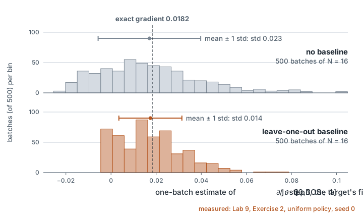Both histograms are centered on the exact gradient from `exact_gradient`; the leave-one-out baseline (Equation 9) cuts the standard deviation from 0.023 to 0.014. The spike at 0 in the lower panel is mostly batches in which no sample wrote that symbol: the leave-one-out weights sum to zero over a batch, so such a batch gives exactly 0. Data: `images/09-baseline-variance.json`; drawn by `scripts/make_figures_09_11.py`.

Credit across tokens. A reward model scores a complete response, so in Equation 6 every token of a response gets the same weight R - b. The reward says the response was good, not which tokens made it good, and only averaging over many samples sorts that out. When a reward arrives after each token instead, each token is weighted by its reward-to-go G_t (Equation 1), and the rewards earned before it, which it could not affect, are dropped. Section 5, for reading after class, derives this and gives the loss code that the lab and Module 10 use.

In the lab. In Exercise 2 you write loo_baseline(returns) (Equation 9); batch_mean_baseline is provided beside it. The checkpoint has two parts. Unbiasedness (Equation 8): averaged over many batches at the uniform starting policy, the estimate with your baseline matches the exact gradient, as the one without a baseline does; and on every batch, the batch-mean estimate equals (1 - 1/N) times yours. Variance: the provided cell measures the total variance of \hat{g} over those batches, without a baseline, with yours, and with the token-level rewards of section 5. Predict the ranking first. A last cell trains several seeds with and without the baseline and prints the steps each needs to reach J \ge 0.9.

Check yourself. A batch of N = 4 responses has rewards (3, 1, 0, 0). Compute the leave-one-out baseline b^{(i)} and the weight R_i - b^{(i)} for each sample. Then compute R_i - \bar{R} with the batch mean, and check the factor the text claims. Which response is made more likely by the update, and which is left alone?

Answer

By Equation 9 the baselines are the means of the other three rewards: (1/3,\ 1,\ 4/3,\ 4/3). The weights are (8/3,\ 0,\ -4/3,\ -4/3). The batch mean is \bar{R} = 1, which gives (2,\ 0,\ -1,\ -1): each is 3/4 = 1 - 1/N of the leave-one-out weight, as claimed. The first response is pushed up and the last two are pushed down. The second, with reward 1, is left alone: it did exactly as well as the others did on average, so it carries no evidence either way. With b = 0 it would have been pushed up, simply for having a positive reward.

5. Generation as Sequential Decisions

Not taught in the room. Lab 9’s Exercise 1 restates the return G_t and the loss it needs; this section explains why a reward that arrives only at the end leaves credit assignment to averaging.

In this section: distinguish a sequence-level reward from token-level rewards, and say what each implies for credit assignment.

Section 3 treated the whole response as one action with one reward. Section 2 described it as T actions with a reward r_t after each. Both views are correct; they differ in where the reward comes from.

Token-level rewards. If a reward arrives after each token, the expected return is J = \mathbb{E}[G_1] (Equation 1), and the same derivation gives

\nabla_\theta J = \mathbb{E}\Big[\sum_{t=1}^{T} \big(G_t - b_t\big)\, \nabla_\theta \log \pi_\theta(y_t \mid s_t)\Big], \qquad G_t = \sum_{t'=t}^{T} r_{t'} , \tag{10}

with b_t any baseline that does not depend on y_t or later tokens. G_t is the reward-to-go: the reward collected from step t onward. The rewards before step t were dropped. They are fixed by the time y_t is drawn, so each one acts as a baseline for step t and contributes zero in expectation, by the per-step form of Equation 7. Dropping them removes noise and keeps the estimate unbiased: the choice of token t is credited only with what came after it.

A sequence-level reward. A reward model, a person, or an exact-match check scores the complete response: r_t = 0 for t < T and r_T = R(x, y). Then G_t = R(x, y) at every step, and with b_t = b, Equation 10 is Equation 4 with a baseline, the gradient of Equation 6 up to its sign: every token of a response gets the same credit, good tokens and bad ones alike. This is the credit-assignment problem: the reward says the response was good, not which tokens made it good. Only averaging over many samples sorts that out.

	Token-level reward	Sequence-level reward
Where it arises	a per-token penalty (Module 10’s KL term), a partial-credit score	a reward model, a person, an exact-match check
Weight on token t	reward-to-go G_t	the same R(x, y) for every t
Credit assignment	partial	none; left to averaging

The rewards of RLHF are mostly sequence-level: the reward model scores a complete response. Treating the whole response as one action, as REINFORCE does, is a sound and simple choice for language models; Ahmadian et al. (2024) report that it matches or beats the per-token treatment of PPO in their experiments.

One function for both. Store the rewards as an (N, T) tensor (for a sequence-level reward, zero except the last column), turn them into returns, and weight each token’s log-probability by its return minus the baseline. This is the code the lab uses, and Module 10 reuses it unchanged:

def returns_to_go(rewards):                  # rewards: (N, T), r_t for each sample
    return rewards.flip(-1).cumsum(-1).flip(-1)        # G_t = r_t + ... + r_T, (N, T)

def reinforce_loss(logp, returns, baseline=0.0):       # logp, returns: (N, T)
    weight = (returns - baseline).detach()              # constants: R is never differentiated
    return -(weight * logp).sum(-1).mean()              # sum over t, mean over samples

def loo_baseline(returns):                   # (N, T) -> (N, T); needs N >= 2
    N = returns.shape[0]
    return (returns.sum(0, keepdim=True) - returns) / (N - 1)   # b_t^(i): mean of the others

Here logp[i, t] is \log \pi_\theta(y^{(i)}_t \mid s^{(i)}_t), so logp.sum(-1) is Equation 2. Responses of different lengths need one more step: zero the padding positions of logp, as the masked loss of Module 7 does, so that only the response’s own tokens, up to and including its end token, are counted.

Optional: Discounting

Many RL texts weight later rewards by \gamma^{t'-t} with a discount factor 0 < \gamma \le 1, so that G_t = \sum_{t' \ge t} \gamma^{t'-t} r_{t'}. Discounting keeps returns finite in episodes with no end and lowers variance at the price of bias. Text episodes are short and always end, and most language-model work uses \gamma = 1, as this module does.

In the lab. The toy task has a natural per-token decomposition, r_t = \mathbf{1}[y_t = y^\star_t] / T, whose sum is the sequence-level reward. The provided third row of the variance table in Exercise 2 feeds these token-level rewards through your returns_to_go (Equation 10), so you compare sequence-level credit with token-level credit on the same samples.

Check yourself. In the toy task, a sampled response matches the target at positions 1, 3 and 6 and misses at 2, 4 and 5. Write the token-level rewards r_t and the returns G_t (Equation 1). What weight does each token get under the sequence-level reward? The token at position 5 was wrong: which scheme gives it less weight, and why is its weight not zero?

Answer

With r_t = \mathbf{1}[y_t = y^\star_t] / 6, the rewards are (\tfrac16, 0, \tfrac16, 0, 0, \tfrac16) and the returns, summing from the right, are G = (\tfrac12, \tfrac13, \tfrac13, \tfrac16, \tfrac16, \tfrac16). The sequence-level reward is R = \tfrac12, and it gives every token the weight \tfrac12. Token 5 gets \tfrac16 under token-level credit against \tfrac12 under sequence-level credit: it is no longer credited with the matches at positions 1 and 3, which were decided before it was drawn. Its weight is not zero because G_5 = r_5 + r_6 includes the match at position 6. The reward-to-go credits a token with everything from its own step onward, and in this task the policy at position 6 conditions on the symbol written at position 5. Its own miss is counted too: had token 5 matched, G_5 would be \tfrac13.

6. Why Comparisons Instead of Scores

In this section: say why preference data is usually collected as comparisons.

You need a reward that only people can give, such as how helpful a response is. Would you ask raters to score each response from 1 to 10, or to say which of two responses is better? Commit to one, and name one way it could go wrong.

The policy gradient needs a reward for any response. For tasks with a checkable answer, a program provides it. For “helpful”, “clear” or “polite”, we need people. The obvious design is to ask raters for a score from 1 to 10. It works poorly, for reasons familiar from any survey:

Raters use the scale differently. One rater’s 6 is another’s 8.
A rater drifts. The same response gets a different score early and late in a session, or after a very good or very bad one.
Absolute judgment is hard; relative judgment is easier. “Which of these two is better?” is a question most people answer quickly and consistently.

So most preference data is collected as comparisons: a prompt x, two responses, and which one the rater preferred. Christiano et al. (2017) trained agents from comparisons of pairs of short video clips; Stiennon et al. (2020) and Ouyang et al. (2022) applied the same idea to language models, with raters comparing or ranking several responses to the same prompt. A ranking of K responses yields \binom{K}{2} pairwise comparisons.

A comparison is a relative label. To use it in the policy gradient we need a number per response. The next section supplies the model that links the two.

7. The Bradley–Terry Model

In this section: write the probability that one response is preferred to another, and state what that model can and cannot identify.

The model. Bradley and Terry (1952) proposed that each item has a latent quality u, and that item a is preferred to item b with probability

P(a \succ b) = \frac{e^{u_a}}{e^{u_a} + e^{u_b}} = \sigma(u_a - u_b). \tag{11}

The second form follows by dividing numerator and denominator by e^{u_a}. It is a softmax over two options (Module 1), and Elo ratings in chess, as commonly implemented, rest on the same model.

A rater with noise. Real raters are inconsistent. We model that with a label temperature \tau_{\text{label}} > 0, which divides the quality gap exactly as the sampling temperature of Module 3 divides the logits:

P(y_a \succ y_b \mid x) = \sigma\Big(\frac{u(x, y_a) - u(x, y_b)}{\tau_{\text{label}}}\Big). \tag{12}

A low temperature is a consistent rater, who almost always prefers the better response. As \tau_{\text{label}} \to \infty the rater flips a coin. Worked example: with \tau_{\text{label}} = 0.5, a gap of u_a - u_b = 1 gives \sigma(2) = 0.88: the better response wins 88 times in 100. Two responses of equal quality each win half the time, whatever the temperature.

What can be identified from comparisons. Three consequences of Equation 12 matter for everything that follows.

Only differences. Adding a constant to every u, or a constant per prompt, leaves every probability unchanged. The level of u is arbitrary.
Scale and noise are tangled. Doubling u and doubling \tau_{\text{label}} gives the same probabilities. From comparisons alone we learn u / \tau_{\text{label}}, never the two separately: a reward learned from noisier raters has smaller differences, not a different ranking.
There is a ceiling on accuracy. The labels are random. Even the true u predicts a held-out label only with probability \max(p, 1 - p), where p is the probability in Equation 12. Over a set of pairs, the best possible pairwise accuracy is

\mathrm{Acc}^\star = \mathbb{E}_{\text{pairs}}\big[\max(p, 1 - p)\big], \qquad p = \sigma\Big(\frac{u(x, y_a) - u(x, y_b)}{\tau_{\text{label}}}\Big). \tag{13}

Pairs of equal quality contribute 0.5. No reward model can beat \mathrm{Acc}^\star on held-out labels from the same raters, except by chance on a small set; one that does so by a wide margin is overfitting or leaking labels.

Optional: Other Comparison Models

Thurstone’s model replaces the sigmoid with the normal cumulative distribution function, which corresponds to Gaussian rather than logistic noise on the qualities. The two give very similar probabilities after rescaling. The Plackett–Luce model extends Bradley–Terry from pairs to full rankings of K items: the top item is chosen by a softmax over all K, the next by a softmax over the rest, and so on. Training on all \binom{K}{2} pairs of a ranking, as InstructGPT did, is a simpler alternative.

In the lab. The second half of Lab 9 uses a synthetic rater whose rule you know, so that you can check what the reward model learns. Prompts are eight-word openings of everyday sentences, such as “My sister opened the letter and felt so”, from a fixed list written for the workshop. Each stops just before a feeling, so the continuations often contain one. The two responses of each pair are 24-token continuations sampled from the small pretrained GPT-2 that you probed in Lab 6 (distilbert/distilgpt2), the model that Lab 10 will fine-tune. The gold score g(y) rewards distinct words from a short list of positive words (counting at most three), subtracts one for each word from a list of negative words, and subtracts a penalty when the response is crowded with words from the two lists. The rater labels each pair with Equation 12, with u = g and a fixed \tau_{\text{label}}. The pairs come with the lab as a data file that stores GPT-2’s token ids and the text of every response, and both gold scores. In Exercise 3 you write bt_prob(g_a, g_b, tau_label); the checkpoint compares your probabilities with the label frequencies in the file, and a provided cell prints \mathrm{Acc}^\star (Equation 13) for the held-out pairs: the ceiling for Exercise 4.

Check yourself. A held-out set has three pairs, with quality gaps u_a - u_b of 0, 1 and 2, labeled by a rater with \tau_{\text{label}} = 0.5. Compute \mathrm{Acc}^\star. A reward model reaches 0.79 on a large held-out set with the same mix of gaps. A colleague calls that mediocre and wants a bigger model. What do you say?

Answer

By Equation 12 the label probabilities are \sigma(0) = 0.5, \sigma(2) \approx 0.881 and \sigma(4) \approx 0.982. Each is already the larger of p and 1 - p, so by Equation 13 \mathrm{Acc}^\star = (0.5 + 0.881 + 0.982) / 3 \approx 0.788. A reward model at 0.79 is at the ceiling: it predicts the labels as well as the true quality u would. The missing 21 points are rater noise and ties, which no model can predict. A bigger model cannot honestly go higher. If it did, by a clear margin on a large set, the first things to check would be overfitting and leaked labels.

8. Training a Reward Model

In this section: write the reward-model loss, connect it to logistic regression, and say what held-out accuracy does and does not tell you.

The reward model. A reward model r_\phi(x, y) is a network with parameters \phi that maps a prompt and a response to one number. In RLHF it is usually a pretrained language model (often the SFT model) whose output layer is replaced by a linear map from the final hidden state to a scalar. InstructGPT’s reward model, for example, was a 6-billion-parameter GPT-3 model with its output layer replaced in this way.

The loss. Replace the latent quality in Equation 11 by r_\phi and maximize the likelihood of the observed comparisons in the dataset \mathcal{D}_{\text{pref}} of triples (x, y_w, y_l):

\mathcal{L}_{\text{RM}}(\phi) = -\frac{1}{|\mathcal{D}_{\text{pref}}|} \sum_{(x,\, y_w,\, y_l) \in \mathcal{D}_{\text{pref}}} \log \sigma\big(r_\phi(x, y_w) - r_\phi(x, y_l)\big). \tag{14}

The label temperature of Equation 12 does not appear: it is absorbed into the scale of r_\phi, as section 7 showed it must be.

def bt_loss(reward_w, reward_l):           # (n,) each: r_phi(x, y_w) and r_phi(x, y_l)
    return -F.logsigmoid(reward_w - reward_l).mean()

F.logsigmoid computes \log \sigma without forming \sigma first, so it neither underflows nor returns \log 0 when the difference is large and negative. Module 10’s DPO loss calls this same function with a different reward.

Worked example: one pair through the loss. For one triple, the reward model gives the preferred response r_\phi(x, y_w) = 1.0 and the other r_\phi(x, y_l) = 0.2. Write \Delta = r_\phi(x, y_w) - r_\phi(x, y_l) for the gap.

Probability (Equation 11): \Delta = 0.8, so the model says the observed preference had probability \sigma(0.8) \approx 0.690.
Loss (Equation 14, one pair): -\log 0.690 \approx 0.371.
Gradient. Since \frac{d}{d\Delta}\big[-\log \sigma(\Delta)\big] = -\sigma(-\Delta), the derivative of the loss is -\sigma(-0.8) \approx -0.310 with respect to r_\phi(x, y_w) and +0.310 with respect to r_\phi(x, y_l). A gradient-descent step raises the winner’s score and lowers the loser’s by the same amount. The two derivatives sum to zero: the loss pulls scores apart and never moves their common level, which is the “only differences” property of section 7.
The same pair, ranked the wrong way. With the scores exchanged, \Delta = -0.8: the loss is -\log \sigma(-0.8) \approx 1.171 and the derivatives have size \sigma(0.8) \approx 0.690. A misranked pair is pushed more than twice as hard as a correctly ranked one.
Before training. If every score is equal, \Delta = 0 and the loss is \log 2 \approx 0.693 for every pair. A reward model whose loss stays near 0.693 has learned nothing.

It is logistic regression. Equation 14 is the binary cross-entropy of Module 1 with the label “the first response wins” and the logit r_\phi(x, y_w) - r_\phi(x, y_l). If the reward were linear in fixed features, r_\phi(x, y) = \phi^\top f(x, y), the logit would be \phi^\top \big(f(x, y_w) - f(x, y_l)\big), and training the reward model would be logistic regression on feature differences, with a convex loss. There is no constant term: a bias cancels in the difference, which is the “only differences” property of section 7 again. A neural reward model is the same loss with learned features.

Fixing the level and scale. Because only differences are identified, a trained reward model has an arbitrary offset. Before handing it to an optimizer, fix it on a reference set of responses with mean \mu and standard deviation \varsigma of the raw scores:

\tilde{r}_\phi(x, y) = \frac{r_\phi(x, y) - \mu}{\varsigma} . \tag{15}

The shift changes nothing in the comparisons. It matters downstream: the policy gradient uses the reward’s level unless a baseline removes it, and Module 10 adds a penalty whose coefficient only makes sense against a reward of known scale.

Evaluation. The standard number is held-out pairwise accuracy: on comparisons not used in training, the share where r_\phi(x, y_w) > r_\phi(x, y_l). Read it against the ceiling \mathrm{Acc}^\star of Equation 13, not against 1. In the lab, where the gold score is known, you can also check directly whether r_\phi ranks held-out responses as g does.

What accuracy does not tell you. Held-out accuracy is measured on responses like those in the training pairs. An optimizer will not stay there: Module 10 searches for the responses with the highest r_\phi, and those can lie where the reward model never saw data and is confidently wrong. This is Goodhart’s law (a measure that becomes a target stops being a good measure), and Gao et al. (2023) measure it for reward models: optimizing harder against a learned reward first raises and then lowers the true reward.

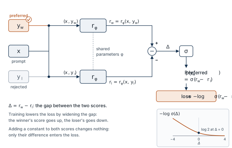
A reward model scores the preferred and the rejected response with shared parameters; the difference of the two scores passes through a sigmoid, and the loss is its negative logarithm. — Figure 3: The reward model and its loss (Equation 14). One network r_\phi, with the same parameters, scores the prompt with the preferred response and with the rejected one; only the difference \Delta = r_\phi(x, y_w) - r_\phi(x, y_l) enters the loss. Inset: the loss -\log \sigma(\Delta) is \log 2 \approx 0.693 when the two scores are equal and falls toward 0 as the preferred response pulls ahead.

In the lab. In Exercise 4 you write bt_loss(reward_w, reward_l) (Equation 14); the checkpoint compares it with hand values and with PyTorch’s binary cross-entropy, and checks that adding a constant to both scores leaves it unchanged. The provided reward model is a small transformer built from the block of Lab 5. It reads GPT-2’s token ids for the prompt and the response together and outputs one number at the last position. Unlike the reward models described at the start of this section, it does not start from a pretrained language model: it is trained from scratch, which keeps Lab 9 on a CPU with no download. One consequence matters in Module 10: it has an embedding only for tokens that occur at least twice in its training pairs, and every other token looks the same to it. After training, three numbers on held-out pairs: pairwise accuracy beside \mathrm{Acc}^\star, accuracy against the ordering by g, and the rank correlation between r_\phi and g. A provided cell then scores a few hand-written responses that the reference model rarely writes, such as one positive word repeated many times or a response made only of positive words, and prints r_\phi beside g: a preview of Module 10. In Exercise 5 you write fit_normalizer(raw_scores) (Equation 15) on the held-out responses and save the reward model, normalization included, to the file that Lab 10 loads. The stretch section raises \tau_{\text{label}} and measures how the reward model’s accuracy degrades as the raters get noisier.

Check yourself. Three reward models score the same pair, preferred response first: model A gives (5.0,\ 3.0), model B gives (105,\ 103) and model C gives (2.5,\ 1.5). All three rank the pair correctly. Which have the same loss on it? Why is C’s loss higher, and is C a worse reward model? What does Equation 15 do to the difference between A and B?

Answer

A and B have the same gap, 2, so the same loss: -\log \sigma(2) \approx 0.127. The level, 5 or 105, never enters Equation 14. C has a gap of 1 and a loss of -\log \sigma(1) \approx 0.313. C is A at half the scale, and by section 7 scale is tangled with rater noise: C describes the same ranking as A with less confident preferences. Which of the two fits better depends on how consistent the raters were, so C is not worse on this evidence. On this pair their pairwise accuracy is identical. Normalization subtracts each model’s own mean on a reference set, which removes an offset such as the 100 between A and B, and divides by each model’s own standard deviation, which removes a factor such as the 2 between A and C. If B were A plus 100 and C were A halved on every response, all three would hand the optimizer exactly the same reward after Equation 15.

Summary

Supervised fine-tuning can only make a given text more likely. It cannot express “better”, imitates its demonstrations, and never trains on the model’s own outputs.
A language model is a policy: the state is the prompt plus the prefix, the action is the next token, and \log \pi_\theta(y \mid x) is a sum over tokens (Equation 2).
The policy gradient (Equation 4) follows from the log-derivative trick. It needs the reward only as a number and the model only through \nabla \log \pi_\theta.
REINFORCE estimates it by sampling (Equation 5). As a loss, it is the negative log-likelihood of the model’s own samples, weighted by reward minus baseline (Equation 6).
The score function has mean zero (Equation 7), so a baseline that does not depend on the sampled response leaves the gradient unbiased (Equation 8) and can cut its variance sharply. The leave-one-out mean is a simple choice (Equation 9); the batch mean shrinks the gradient by 1 - 1/N.
With token-level rewards, each token is weighted by its reward-to-go (Equation 10). With a sequence-level reward every token gets the same credit, and averaging does the assignment.
Preferences are collected as comparisons, because people compare more consistently than they score.
Bradley–Terry turns qualities into preference probabilities (Equation 11, Equation 12). Only differences are identified, scale is tangled with rater noise, and held-out accuracy has a ceiling (Equation 13).
A reward model is trained with the pairwise logistic loss (Equation 14), is normalized before use (Equation 15), and is only trustworthy on data like its training data.

Equations and Where You Implement Them

Equation	Lab 9
Sequence log-probability (Equation 2)	provided: `token_logprobs(logits, actions)`, summed over t
Return and reward-to-go (Equation 1)	Exercise 1: `returns_to_go(rewards)`
Expected reward and its exact gradient (Equation 3, Equation 4)	provided: `exact_gradient(theta)`, by enumeration of the 8^6 toy responses
REINFORCE estimate and loss (Equation 5, Equation 6)	Exercise 1: `reinforce_loss(logp, returns, baseline=0.0)`; the checkpoint compares its mean gradient with `exact_gradient`
Two-action variance example (section 4)	not implemented; Exercise 2 measures the same effect on the toy task
Score has mean zero; baseline leaves the mean unchanged (Equation 7, Equation 8)	Exercise 2 checkpoint: mean estimates with and without a baseline against `exact_gradient`
Leave-one-out and batch-mean baselines (Equation 9)	Exercise 2: `loo_baseline(returns)`; provided: `batch_mean_baseline(returns)`
Token-level credit (Equation 10)	provided: third row of the Exercise 2 variance table, using your `returns_to_go`
Bradley–Terry with a label temperature (Equation 11, Equation 12)	Exercise 3: `bt_prob(g_a, g_b, tau_label)`, checked against the labels in the pairs file
Accuracy ceiling (Equation 13)	provided: `oracle_accuracy(g_a, g_b, tau_label)`, printed in Exercise 3 and beside the Exercise 4 result
Reward-model loss (Equation 14)	Exercise 4: `bt_loss(reward_w, reward_l)`; provided: the `RewardModel` class and its training loop
Normalization (Equation 15)	Exercise 5: `fit_normalizer(raw_scores)`; saved with the model for Lab 10
Accuracy against rater noise (section 7)	Stretch
Actor-critic baselines, discounting, Plackett–Luce (optional callouts)	not implemented in this lab

Gotchas and Troubleshooting

“The reward has to be differentiable.” It never is differentiated. Equation 4 needs only its value.
“The policy-gradient loss tells you how training is going.” Equation 6 is a device for producing the right gradient. Its value depends on the baseline and moves for reasons unrelated to progress. Monitor the mean reward.
“A baseline changes what the policy converges to.” In expectation it changes nothing (Equation 8). It only changes the noise, though less noise can keep training from stalling.
“Any baseline is fine.” It must not depend on the response it is subtracted from. The leave-one-out mean qualifies; a baseline that includes the sample’s own reward shrinks the gradient.
“RL for language models needs per-token rewards and PPO.” A sequence-level reward with REINFORCE and a good baseline is a sound method; Module 10 places PPO in context.
“A reward model outputs how good a response is.” It outputs a number whose differences are meaningful. Its level is arbitrary and its scale reflects the raters’ noise as much as quality.
“A reward model should reach 100% held-out accuracy.” Raters are noisy and many pairs are close; the ceiling is \mathrm{Acc}^\star (Equation 13), often well below 1.
“An accurate reward model is a safe objective.” Its accuracy is measured on the data it was trained on. An optimizer leaves that data, and Module 10 shows what happens then.
“Preferences measure truth.” They measure what raters prefer. Whether that is what we want is a question for Modules 10 and 12.

Next Steps

You can now optimize a policy against any reward with the policy gradient, and you can learn a reward from comparisons. Module 10 joins them into reinforcement learning from human feedback: the pretrained GPT-2 whose samples made up this lab’s pairs is fine-tuned against the reward model you saved, with a penalty that keeps it close to where it started. It then removes the penalty to watch the reward model’s blind spots get exploited, and introduces DPO, which learns from the same comparisons without a separate reward model or a sampling loop.