Fine-Tuning and LoRA

Day 2 · Transformers and Pretraining Module 7 120 minutes (55 briefing, 55 lab, 10 debrief) 14:45 briefing · 15:40 lab · 16:35 debrief

Turning a pretrained language model into an instruction follower, efficiently.

Open the lab in Colab Hugging Face PEFT PyTorch

Duration

120 minutes (55 briefing, 55 lab, 10 debrief)

Level

300 · Advanced

Lab runtime

Google Colab, free T4 GPU · about 7 minutes of compute

Accounts and cost

Google. Free

Without API keys

an open model runs in place of the commercial one

What You Will Build

In this module you will:

• Turn a pretrained causal LM into an instruction follower
• Apply LoRA and explain why it works
• Choose decoding settings and evaluate generated text

New terms, in the glossary: chat template, LoRA (low-rank adaptation).

Before You Start

• Module 6 · Pretraining and the Hugging Face Stack and its lab, and the modules before it: this module measures its results against theirs.
• A Google account, and the Colab runtime set to T4 GPU (Runtime → Change runtime type).
• API keys are optional. Without them an open model runs in place of the commercial one.

Where we are. Module 6 ended with a pretrained causal language model that continues text, and with a fine-tuning recipe that updates every parameter. Neither is enough for an assistant: the model cannot tell a request from a reply, and updating every weight does not scale. This module answers one question: how do we teach a pretrained model to follow instructions while training well under 1% of its parameters?

In the Lab

Open the lab in Colab

6 exercises in 4 parts. The notebook budgets 50 minutes for them; the lab slot is 55 minutes. Each exercise you write is a # TODO stub with a folded solution beneath it and a checkpoint that passes or fails; where people tend to stall, a folded hint sits above the stub.

Task	Briefing section	Time
Step 0 · A Language Model Continues; It Does Not Answer	—	3 min
Part A · LoRA by Hand
Exercise 1 · The LoRA Layer	5	10 min
Exercise 2 · Merging the Update	5	5 min
Part B · Instruction Data
Exercise 3 · The Chat Template	2	6 min
Exercise 4 · The Response Mask and the Labels	3	8 min
Part C · LoRA With peft
Exercise 5 · Configure LoRA and Count Its Parameters	6	10 min
Part D · Decoding and Evaluating Generated Text
Exercise 6 · ROUGE-n and Decoding Settings	7, 8	8 min

Challenge · How Large a Rank?

Optional, for anyone who finishes the core path early: the notebook’s stretch section, after the last checkpoint.

When you are done. Runtime → Disconnect and delete runtime releases the machine; your keys stay in Colab Secrets for the next lab.

Agenda

Minutes	Section	In the room
0–4	1. A Language Model Continues; It Does Not Answer	—
4–9	2. Chat Templates	—
9–17	3. The Instruction-Tuning Loss	Check yourself (2 min)
17–21	4. What Full Fine-Tuning Costs	Predict (1 min)
21–39	5. LoRA: A Low-Rank Update	Demo (4 min); Check yourself (2 min)
39–45	6. LoRA in Practice: Where, How Large, and the peft Library	—
45–48	7. Decoding Settings	—
48–55	8. Evaluating Generated Text	Check yourself (2 min)
55	Total	44 minutes of exposition, 11 of activities

Checks, demos and predictions listed here are part of the live session and its minutes; the others on the page are for reading afterwards.

Read now · Sections 1–8, in the agenda above.

Use in the lab · Exercises 1 and 2: section 5; Exercise 3: section 2; Exercise 4: section 3; Exercise 5: section 6; Exercise 6: sections 7 and 8.

Read later · The collapsed callouts marked Optional; Further Reading.

1. A Language Model Continues; It Does Not Answer

In this section: state what a pretrained causal language model lacks as an assistant, and what fine-tuning must add.

Module 6 left us with a pretrained causal language model: a decoder-only transformer trained to predict the next token of ordinary text. Give it a prefix and it writes a plausible continuation.

That is not the same as doing what the prefix asks. Given the request Name the capital of France. and decoded greedily, the lab’s pretrained model, before any fine-tuning, writes something of this kind:

Name the capital of France.

The French are a very proud people. They are very proud of their
history and their culture. ...

This output is illustrative, written to show the pattern; it is not a recorded run. Step 0 of the lab shows you the model’s real output on five held-out prompts. The pattern to look for: it repeats the request, drifts into unrelated text, and does not stop before the length limit. This is likely text, which is all the model was trained to produce. It is not an answer followed by a stop. The model has no notion of who is speaking, of whose turn it is, or of when a reply is finished.

Module 6 also showed the standard remedy for a mismatch between pretraining and the task: fine-tuning, which continues training on task data. There you updated every weight of a small encoder. Two things are open:

1. What is the task data here, and what is the loss? We want an instruction follower: a model that reads a request and writes a reply to it. Sections 2 and 3 show that this needs no new architecture and no new loss, only formatted data and a mask.
2. Updating every weight is expensive, and it gets worse with model size. Sections 4 to 6 derive LoRA (low-rank adaptation), which trains well under 1% of the parameters.

Sections 7 and 8 then deal with the output: how to generate from the tuned model, and how to say with a number whether the text it writes is any good.

Optional: Pretraining, Full Fine-Tuning and LoRA Compared

The three ways of training that Modules 6 and 7 use, side by side. Read it now as a map of the module, or after section 6 as a summary.

	Pretraining (Module 6)	Full fine-tuning (Module 6, section 7)	Instruction tuning with LoRA (this module)
Data	a very large corpus of plain text, with no labels	labeled task data: arXiv abstracts and their topics	instruction–response pairs, formatted with the chat template (section 2)
Loss	self-supervised: next-token (causal) or masked-token cross-entropy	cross-entropy of a new classification head	next-token cross-entropy on the response tokens only (Equation 1)
What is updated	every parameter	every parameter, the pretrained body and the new head, at a small learning rate	only the adapter A and B; W_0 is frozen (Equation 3)
Where training starts	random weights	\theta_{\text{pre}}, with a random head	exactly the pretrained model, because B = 0
What is kept per task	one model, reused by every task	a full copy of the model	the adapter: a few megabytes (section 6)
Typical failure	as an assistant, it continues the prompt instead of answering, and does not stop (this section)	memory for a gradient and optimizer state on every weight, and a small dataset that pulls the model away from what pretraining learned (section 4)	too low a rank for a task far from the pretraining data (section 5); a closing token left out of the loss, so the model never learns to stop (section 3)

Check yourself. Apply the table to a new task. A team has a pretrained causal LM and 2,000 support tickets, each with the reply an agent sent. Run 1 trains every weight with the next-token loss on the whole formatted conversation, ticket included. Run 2 trains a LoRA adapter on q_proj and v_proj with the response mask of section 3. For each run, which weights change, which positions are in the loss, and what is saved at the end? Run 1’s training loss is lower than run 2’s. Does that show that it writes better replies?

Answer

Run 1 changes every weight, scores every position (the ticket, the role names and the reply), and saves a full copy of the model; during training it holds a gradient and optimizer state for every weight. Run 2 changes only A and B in the targeted layers, scores only the reply tokens and the closing <|im_end|>, and saves only the adapter; W_0 is unchanged, and the adapter can be merged into it afterwards. The two training losses are averages over different positions, so they cannot be compared, and run 1’s includes the ticket text, which is not what the team wants the model to learn. Compare the two runs on held-out examples with the response perplexity (Equation 2), over the same scored positions, and read the replies they generate.

2. Chat Templates

In this section: write a conversation as the single string the model sees.

A causal language model takes one sequence of tokens. A conversation is a list of messages, each with a role (system, user or assistant) and a content string. A chat template is the function that turns the list into one string. It is plain string formatting, with special tokens marking where each message starts and ends. A special token is a vocabulary entry reserved for structure: the tokenizer never produces it from ordinary text, so the model can tell markup from content.

The lab uses the ChatML layout. It has two special tokens: <|im_start|> opens a message and <|im_end|> closes it. The whole template is this function:

def format_chat(messages, add_generation_prompt=False):
    text = ""
    for m in messages:   # m = {"role": ..., "content": ...}
        text += "<|im_start|>" + m["role"] + "\n" + m["content"] + "<|im_end|>\n"
    if add_generation_prompt:
        text += "<|im_start|>assistant\n"
    return text

A training example, one instruction and its reference response, becomes:

<|im_start|>user
Name the capital of France.<|im_end|>
<|im_start|>assistant
Paris.<|im_end|>

At generation time there is no assistant message yet. We format the user message and append the opening of an assistant message, <|im_start|>assistant\n. This suffix is the generation prompt. The most likely continuation is now a reply, and the reply ends when the model emits <|im_end|>, which we use as the stop token (section 7 adds a second one).

In Hugging Face transformers the template is stored with the tokenizer as a Jinja string (Jinja is a small templating language) and applied with apply_chat_template:

tokenizer.chat_template = (
    "{%- for message in messages %}"
    "{{- '<|im_start|>' + message['role'] + '\n' + message['content'] + '<|im_end|>' + '\n' }}"
    "{%- endfor %}"
    "{%- if add_generation_prompt %}{{- '<|im_start|>assistant\n' }}{%- endif %}"
)

messages = [{"role": "user", "content": "Name the capital of France."}]
prompt = tokenizer.apply_chat_template(messages, tokenize=False, add_generation_prompt=True)

Three points to carry away:

• The template is part of the model. A model fine-tuned with one layout expects exactly that layout, down to the newlines. With the wrong template it still produces text, only worse. This is why the template is saved with the tokenizer.
• Use add_generation_prompt=False for training text and True for generation. A training example already contains the assistant message.
• Do not add special tokens twice. The template writes all the special tokens it needs. If you format to a string and tokenize it afterward, pass add_special_tokens=False.

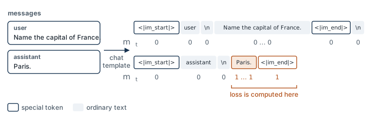
Figure 1: A two-message conversation formatted with the ChatML template, and the response mask m_t of Equation 1. Special tokens are outlined. Only the response and its closing <|im_end|> have m_t = 1, so only they are scored.

In the lab. In Exercise 3 you write format_chat and check that it returns exactly the string that tokenizer.apply_chat_template returns for the same messages.

Check yourself. At generation time you call format_chat(messages) on one user message and forget add_generation_prompt=True. Write the last line of the string the model receives. What is it now free to write next, and why is that a problem?

Answer

The string ends with the user’s message and its closing token: Name the capital of France.<|im_end|> and a newline. Nothing says whose turn is next, so the model must write <|im_start|> and a role name itself. It may write assistant, or it may write user and continue with a second user message. Whatever follows is returned to you as “the reply”. The generation prompt removes that choice: it fixes the next speaker, so the only thing left to predict is the reply.

3. The Instruction-Tuning Loss

In this section: write the loss that turns a language model into an instruction follower.

Instruction tuning is fine-tuning on pairs of an instruction and a good response, each formatted with the chat template. The model, the objective and the optimizer are those of Modules 3, 5 and 6. One thing changes: which positions are scored.

Let w_1, \dots, w_T be the tokens of one formatted example, with T its length, and let w_{<t} abbreviate w_1, \dots, w_{t-1}. Define a response mask m_t \in \{0, 1\} for each position:

• m_t = 1 if w_t is a token of the assistant’s response, including the closing <|im_end|>;
• m_t = 0 otherwise: the instruction, the role names and the generation prompt.

A training sequence stops at the closing <|im_end|> of the response. The template writes a newline after it, but generation stops at <|im_end|>, so the model never has to produce that newline: it is dropped from the sequence and never scored.

The instruction-tuning loss is the mean negative log-likelihood over the response positions only:

\mathcal{L}_{\text{resp}}(\theta) = -\frac{1}{\sum_{t=1}^{T} m_t} \sum_{t=1}^{T} m_t \log P_\theta(w_t \mid w_{<t}), \tag{1}

where \theta denotes the trainable parameters. With m_t = 1 everywhere this is the language-model loss of Module 3.

Why mask?

• The instruction is the condition, not the target. We want P_\theta(\text{response} \mid \text{instruction}). This is the conditional language model of Module 4: the instruction plays the part of the source, the response the part of the target, and both now sit in one sequence. The model still reads the instruction tokens, because every response token is conditioned on them through w_{<t}. They are only left out of the sum.
• Capacity and signal. Unmasked, part of every gradient step is spent on predicting what users write. For short responses to long instructions, that part dominates.
• The closing token is in the sum on purpose. It is how the model learns to stop.

The matching evaluation number is the response perplexity, the perplexity of Module 3 restricted to the same positions:

\mathrm{PPL}_{\text{resp}} = \exp\big(\mathcal{L}_{\text{resp}}\big), \tag{2}

with \mathcal{L}_{\text{resp}} averaged over all response tokens of a held-out set. Module 3’s conditions for comparing perplexities hold between the model before and after fine-tuning: same tokenizer, same text, same scored positions.

In code, the mask is applied through the labels. PyTorch’s cross-entropy skips every position whose label equals its ignore_index, which is -100 by default, and Hugging Face models follow that convention:

def build_labels(input_ids, response_mask):     # both (batch_size, T)
    labels = input_ids.clone()                  # the model still reads every token
    labels[response_mask == 0] = -100           # prompt and padding are not scored
    return labels

labels = build_labels(input_ids, response_mask)
loss = model(input_ids=input_ids, attention_mask=attention_mask, labels=labels).loss

Padding positions have m_t = 0, so they also get -100. The model shifts the labels by one position itself: the label at position t is scored against the prediction made at t - 1.

In the lab. In Exercise 4 you write build_labels for Equation 1; the provided encode_example builds response_mask. The checkpoint counts the scored positions on a known example and compares the model’s loss with a hand computation. The provided response_loss reports Equation 1 on held-out examples, and Equation 2 is its exponential.

Check yourself. A formatted example has 10 tokens. Three of them are the response: two words and the closing <|im_end|>. The model gives these three the probabilities 0.5, 0.25 and 0.5. Compute \mathcal{L}_{\text{resp}} and \mathrm{PPL}_{\text{resp}}. Why do you not need the other seven probabilities? What would the model fail to learn if the mask on the closing token were 0?

Answer

\mathcal{L}_{\text{resp}} = \tfrac{1}{3}(\log 2 + \log 4 + \log 2) = \tfrac{4}{3}\log 2 \approx 0.924, and \mathrm{PPL}_{\text{resp}} = e^{0.924} \approx 2.52. The other seven positions have m_t = 0, so they enter neither the sum nor the count of Equation 1. The model still reads them: each response probability is conditioned on them. With the closing token masked out, no training step would ever reward writing <|im_end|> after an answer. The model would answer and then keep writing until the length limit.

4. What Full Fine-Tuning Costs

In this section: say where the cost of updating every weight comes from.

A model with 7 billion parameters, stored at 4 bytes each, takes 28 GB. How much memory does full fine-tuning with Adam need before a single activation is stored: about 28 GB, about 56 GB, or more? What else has to be kept for every weight?

Full fine-tuning updates all N parameters of the model. Three costs follow.

• Memory during training. Besides the weights, training stores one gradient per trainable parameter, and the Adam optimizer keeps two running averages per trainable parameter. That is about four numbers per parameter in total. At 4 bytes per number, a model with 7 billion parameters needs about 4 \times 4 \times 7 \times 10^9 bytes = 112 GB before a single activation is stored. A free Colab T4 has 16 GB.
• Storage and serving. Each fine-tuned task yields a full copy of the model. Ten tasks are ten copies to store and to load.
• Overwriting. Every weight is free to move, and a small dataset can pull the model away from what it learned in pretraining.

Parameter-efficient fine-tuning (PEFT) is the family of methods that freeze the pretrained weights and train a small number of new parameters. A frozen parameter needs no gradient and no optimizer state, and what must be stored per task is only the small new part. LoRA is the most widely used of these methods.

One caveat. The activations of the forward pass must still be kept to backpropagate through the frozen layers to the trainable ones, so memory falls by less than the parameter count does. Hu et al. (2022) report 10,000 times fewer trainable parameters but 3 times less GPU memory for GPT-3.

Check yourself. The lab’s model has 134.5 million parameters, and its LoRA adapter trains 460,800 of them (section 6 derives that number). With the rule above, four numbers per trainable parameter and one per frozen parameter at 4 bytes each, estimate the parameter-related training memory for full fine-tuning and for LoRA. LoRA trains about 290 times fewer parameters. Does memory fall 290-fold?

Answer

Full fine-tuning: 4 \times 4 \times 134.5 \times 10^6 bytes \approx 2.15 GB. LoRA: the frozen weights still take 4 \times 134.5 \times 10^6 bytes \approx 0.54 GB, and the adapter, with its weights, gradients and optimizer state, adds 4 \times 4 \times 460{,}800 bytes \approx 7.4 MB. So this part of the memory falls about 4-fold, not 290-fold, because the frozen weights still have to be held. The activations, which neither estimate counts, shrink even less. This is the gap between 10,000 times and 3 times in the paper’s GPT-3 figures.

5. LoRA: A Low-Rank Update

In this section: derive the LoRA layer: its form, its initialization, its parameter count and its merge.

Setup. Take one linear layer of the pretrained model, with weight matrix W_0 \in \mathbb{R}^{d_{\text{out}} \times d_{\text{in}}}. It maps an input x \in \mathbb{R}^{d_{\text{in}}} to an output h = W_0 x \in \mathbb{R}^{d_{\text{out}}} (plus a bias, which stays frozen and is omitted below). Fine-tuning replaces W_0 by W_0 + \Delta W, where \Delta W is the update: everything training changed. In full fine-tuning \Delta W is an arbitrary d_{\text{out}} \times d_{\text{in}} matrix.

The idea. LoRA (Hu et al., 2022) restricts \Delta W to be a product of two thin matrices, and trains only those:

W = W_0 + \frac{\alpha}{r}\, B A, \qquad B \in \mathbb{R}^{d_{\text{out}} \times r}, \quad A \in \mathbb{R}^{r \times d_{\text{in}}}, \tag{3}

where

• r is the rank, a small integer chosen by us (1 to 64 is typical), with r \ll \min(d_{\text{in}}, d_{\text{out}});
• A projects the input down to r dimensions and B projects back up to d_{\text{out}};
• \alpha > 0 is a fixed scaling constant, also chosen by us; it is not trained;
• W_0 is frozen: it receives no gradient. The trainable parameters are \theta = (A, B).

The forward pass adds a bypass around the frozen layer:

h = W_0 x + \frac{\alpha}{r}\, B (A x). \tag{4}

The product BA has the shape of W_0, and its rank is at most r, because every output of BAx lies in the span of the r columns of B. The pair (A, B) is called an adapter.

Notation. Three clashes, resolved for this module.

• \alpha. In Modules 4 and 5, \alpha with position subscripts, as in \alpha_{t,i}, is an attention weight. In this module \alpha with no subscript is LoRA’s scaling constant, a single number. In code it is lora_alpha.
• A and B. We keep the letters of the LoRA paper because the peft library names its tensors lora_A and lora_B. In this module A and B are always the LoRA matrices. A is not Module 5’s matrix of attention weights. B is not the batch size of Module 3’s code shapes or the beam size of Module 4; batch size is written out in words here.
• r is the LoRA rank, a different quantity from the frequency rank in Module 1’s Zipf plot.

Figure 2: A LoRA layer (Equation 4). The frozen W_0 and a low-rank bypass run in parallel: A maps the input down to r numbers and B maps them back up to d_{\text{out}}, scaled by \alpha / r. Only A and B are trained; B starts at zero, so the layer starts as W_0.

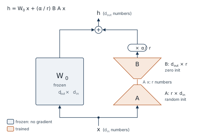
Parameter count. A has r \times d_{\text{in}} entries and B has d_{\text{out}} \times r, so one adapted layer trains

r\,(d_{\text{in}} + d_{\text{out}}) \quad \text{parameters, in place of} \quad d_{\text{in}}\, d_{\text{out}}. \tag{5}

The count grows with the sum of the dimensions, not the product. In the lab’s model the query projection of an attention block has d_{\text{in}} = d_{\text{out}} = 576: that is 576 \times 576 = 331{,}776 frozen weights, and with r = 8 the adapter has 8 \times (576 + 576) = 9{,}216 parameters, 2.8% of the layer. Since only some layers are adapted, the share of the whole model is far smaller (section 6).

Initialization. A is set to small random values and B to zero. Two consequences:

1. Training starts at the pretrained model. With B = 0 the product BA is zero, so W = W_0 exactly and Equation 4 gives h = W_0 x. The first forward pass is the pretrained model’s, not a perturbed one.
2. Training can still start. Let g = \partial \mathcal{L} / \partial h \in \mathbb{R}^{d_{\text{out}}} be the gradient of the loss with respect to the layer’s output. Applying the chain rule to Equation 4:

\frac{\partial \mathcal{L}}{\partial B} = \frac{\alpha}{r}\, g\, (A x)^\top, \qquad \frac{\partial \mathcal{L}}{\partial A} = \frac{\alpha}{r}\, (B^\top g)\, x^\top . \tag{6}

Check the shapes: g\,(Ax)^\top is d_{\text{out}} \times r, like B; (B^\top g)\, x^\top is r \times d_{\text{in}}, like A. At initialization B = 0, so the gradient for A is zero, but Ax \neq 0, so the gradient for B is not. The first step moves B away from zero; from then on A receives gradient too.

If both matrices started at zero, both gradients in Equation 6 would be zero and nothing would ever move. Setting A = 0 and B random would work by the same argument with the roles exchanged; B = 0 is the convention of the paper and of peft.

The scale \alpha / r. The constant multiplies the update, and by Equation 6 it multiplies both gradients, so it acts much like a learning-rate multiplier for the adapter. Dividing by r keeps the size of the update roughly comparable when you change the rank, so that a rank sweep does not need a new learning rate for each rank. A common starting point is \alpha = 2r or \alpha = r; treat it as a hyperparameter of the same kind as the learning rate.

Merging. After training, Equation 3 is just a matrix of the same shape as W_0. Compute it once and store it in place of W_0:

W_{\text{merged}} = W_0 + \frac{\alpha}{r}\, B A \quad \Longrightarrow \quad W_{\text{merged}}\, x = W_0 x + \frac{\alpha}{r}\, B A x \quad \text{for every } x . \tag{7}

The merged layer is an ordinary linear layer: no extra parameters, no extra computation, no added latency at inference. Subtracting \frac{\alpha}{r} BA restores W_0. The alternative is to keep one copy of the base model and swap small adapters in and out, one per task.

Worked example: a LoRA layer by hand. Take d_{\text{in}} = 3, d_{\text{out}} = 2, rank r = 1 and \alpha = 2, so the scale is \alpha / r = 2. Suppose that after some training

W_0 = \begin{pmatrix} 1 & 0 & 2 \\ 0 & 1 & -1 \end{pmatrix}, \qquad A = \begin{pmatrix} 1 & -1 & 0 \end{pmatrix}, \qquad B = \begin{pmatrix} 0.5 \\ -1 \end{pmatrix}, \qquad x = \begin{pmatrix} 2 \\ 1 \\ 1 \end{pmatrix}.

• Frozen path: W_0 x = (4,\ 0)^\top.
• Bypass (Equation 4): Ax = 2 - 1 + 0 = 1, a single number because r = 1. Then B(Ax) = (0.5,\ -1)^\top, and after the scale, (1,\ -2)^\top.
• Output: h = (4,\ 0)^\top + (1,\ -2)^\top = (5,\ -2)^\top.
• Merge (Equation 7): BA = \begin{pmatrix} 0.5 & -0.5 & 0 \\ -1 & 1 & 0 \end{pmatrix}, so W_{\text{merged}} = W_0 + 2BA = \begin{pmatrix} 2 & -1 & 2 \\ -2 & 3 & -1 \end{pmatrix}, and W_{\text{merged}}\, x = (4 - 1 + 2,\ -4 + 3 - 1)^\top = (5,\ -2)^\top. The same output, from one ordinary matrix.
• Rank: both rows of BA are multiples of the one row of A. That is what rank 1 means: the update can move the output along a single direction, the column of B.
• Count (Equation 5): r\,(d_{\text{in}} + d_{\text{out}}) = 5 trained numbers, against 6 in W_0. At this size nothing is saved. The saving comes with width: at d_{\text{in}} = d_{\text{out}} = 576 and r = 8 it is 9,216 against 331,776.

Demo: the sum against the product.

Predict first. At a fixed rank r, what happens to the adapter’s share of the layer when the width d doubles? And at which rank does the adapter have as many parameters as the frozen matrix itself?

viewof d07 = Inputs.range([64, 4096], {label: "Width d (d_in = d_out)", step: 64, value: 576})
viewof r07 = Inputs.range([1, 64], {label: "Rank r", step: 1, value: 8})
viewof alpha07 = Inputs.range([1, 128], {label: "Scaling constant α", step: 1, value: 16})

Plot.plot({
  width: 720, height: 320, marginLeft: 70, grid: true,
  x: {type: "log", label: "width d"},
  y: {type: "log", label: "parameters in one layer"},
  color: {legend: true, domain: ["frozen W0: d × d", "LoRA adapter: r (d + d)"], range: ["var(--demo-blue)", "var(--demo-orange)"]},
  marks: [
    Plot.line(curve07, {x: "d", y: "n", stroke: "kind", strokeWidth: 2}),
    Plot.ruleX([d07], {stroke: "var(--demo-grey)", strokeDasharray: "4 3"}),
    Plot.dot([{d: d07, n: d07 * d07, kind: "frozen W0: d × d"}, {d: d07, n: 2 * r07 * d07, kind: "LoRA adapter: r (d + d)"}],
      {x: "d", y: "n", fill: "kind", r: 5})
  ]
})

curve07 = Array.from({length: 64}, (_, i) => 64 * (i + 1)).flatMap(d => [
  {d, n: d * d, kind: "frozen W0: d × d"},
  {d, n: 2 * r07 * d, kind: "LoRA adapter: r (d + d)"}
])

html`<p>Frozen matrix: <strong>${(d07 * d07).toLocaleString("en-US")}</strong> parameters. Adapter: <strong>${(2 * r07 * d07).toLocaleString("en-US")}</strong>, which is <strong>${(100 * 2 * r07 / d07).toFixed(2)}%</strong> of the layer. Scale α / r = <strong>${(alpha07 / r07).toFixed(2)}</strong>.</p>`

The demo plots both sides of Equation 5 for a square layer, on logarithmic axes. The frozen matrix grows as d^2 and the adapter as 2rd, so the adapter’s share is 2r / d: it halves each time the width doubles, and it reaches 100% at r = d / 2, where LoRA stops saving anything. The last number is the scale of Equation 3: raising r with \alpha fixed shrinks it, which is why \alpha is usually set in proportion to r.

The whole layer in code:

class LoRALinear(nn.Module):
    def __init__(self, base: nn.Linear, r: int, alpha: float):
        super().__init__()
        self.base = base
        for p in self.base.parameters():
            p.requires_grad_(False)                        # freeze W_0 and the bias
        d_out, d_in = base.weight.shape
        self.A = nn.Parameter(torch.randn(r, d_in) * 0.01)  # (r, d_in), small random
        self.B = nn.Parameter(torch.zeros(d_out, r))        # (d_out, r), zero
        self.scale = alpha / r

    def forward(self, x):                                   # x: (..., d_in)
        return self.base(x) + self.scale * (x @ self.A.T @ self.B.T)


def merged_weight(layer):                                   # (d_out, d_in)
    return layer.base.weight + layer.scale * (layer.B @ layer.A)

LoRALinear.merged_weight = merged_weight                    # attach it as a method

The lab writes merged_weight as a separate function and attaches it to the class, so that Exercise 2 can come after a training cell without redefining LoRALinear.

Why should a low-rank update be enough? Three parts, in decreasing order of certainty.

• Nothing is lost at the start. The model begins at W_0 with all of its pretrained ability and only has to learn the change.
• The change needed is often small. Instruction tuning does not teach the language again. It teaches a format and a behavior. Hu et al. hypothesize that the update needed for adaptation has low “intrinsic rank”, building on Aghajanyan et al. (2021), who showed that pretrained models can be fine-tuned well within a subspace of surprisingly few dimensions.
• This is an empirical finding, not a theorem. A rank-r matrix cannot represent an arbitrary \Delta W. When the target task is far from the pretraining data, or the model must absorb much new knowledge, a low rank can underperform full fine-tuning. The rank sweep in the lab’s stretch section is how you find out for a given task.

In the lab. Exercise 1 is the layer: you write the initialization and the forward pass of LoRALinear (Equation 3, Equation 4). Two checkpoints: the output equals the base layer’s output at initialization, because B = 0; and the number of trainable parameters equals r(d_{\text{in}} + d_{\text{out}}) (Equation 5). In Exercise 2 you write merged_weight (Equation 7), after a provided loop has trained a layer on a toy regression so that B is nonzero, and check that a plain linear layer with the merged weight reproduces the adapter’s output to floating-point tolerance. The gradients of Equation 6 are computed by autograd; a provided cell prints them at initialization so you can see that the gradient of A is zero and that of B is not.

Check yourself. A colleague initializes both A and B with small random values, “so that both get a gradient from the first step”. Does training still work? What has been lost?

Answer

Training works: by Equation 6 both gradients are now nonzero at step 1. What is lost is the starting point. With B \neq 0 the product BA is not zero, so W = W_0 + \frac{\alpha}{r} BA \neq W_0: the first forward pass runs a randomly perturbed copy of the pretrained model, in every adapted layer at once. Zero-initializing B costs nothing, since B still gets a gradient, and it guarantees that step 0 is exactly the pretrained model.

Check yourself. You train with r = 8 and \alpha = 16. For a second run you raise the rank to r = 16 and leave everything else alone. What happened to the scale in Equation 3, and what would you set \alpha to if you wanted to change only the rank?

Answer

The scale \alpha / r fell from 16 / 8 = 2 to 16 / 16 = 1. By Equation 6 the scale also multiplies both gradients, so the second run differs from the first in two ways: more capacity, and a smaller effective step for the adapter. To change only the rank, keep the ratio and set \alpha = 32. This is the practical meaning of “\alpha is tuned like a learning rate”: when you report a rank sweep, report \alpha with it.

6. LoRA in Practice: Where, How Large, and the peft Library

In this section: choose target modules and a rank, and read a LoraConfig.

Which layers. Equation 3 applies to any linear layer. A transformer block (Module 5) has several: the query, key, value and output projections of attention, and the two layers of the feed-forward network. Hu et al. adapted only the query and value projections and found that, for a fixed parameter budget, spreading a small rank over both worked better than a large rank on one. Adapting every linear layer costs more parameters and often helps on harder tasks. The lab starts with query and value, named q_proj and v_proj in its model.

How large. In the lab’s model, 30 blocks each have a q_proj of shape 576 \times 576 and a v_proj of shape 192 \times 576. With r = 8, Equation 5 gives 8 \times (576 + 576) + 8 \times (576 + 192) = 15{,}360 parameters per block and 460{,}800 in total, about 0.34% of the model’s 134.5 million. You will check this number in the lab.

Adapting every linear layer of every block at r = 8 trains 2{,}442{,}240 parameters, about 1.8% of the model and 5.3 times as many. Whether the query-and-value adapter is enough for this model to learn to end its replies with <|im_end|> within the lab’s step budget is an open question: we have not yet measured it on the real model. The lab’s stretch section measures it, reporting how replies end for both choices.

Which rank. Small ranks go a long way. Raising r adds capacity and parameters in proportion; past some point quality stops improving. There is no formula for that point. Sweep it.

The library. Hugging Face peft wraps the targeted layers of a model with the layer of section 5:

from peft import LoraConfig, get_peft_model

config = LoraConfig(
    r=8,                                   # the rank r
    lora_alpha=16,                         # the constant alpha; the scale is lora_alpha / r
    target_modules=["q_proj", "v_proj"],   # every module whose name ends with one of these
    task_type="CAUSAL_LM",
)
model = get_peft_model(base_model, config)   # freezes the base weights, adds A and B
model.print_trainable_parameters()           # trainable params, all params, trainable %

# ... train with the loss of section 3 ...

model.save_pretrained("lab07-adapter")       # writes only the adapter: a few megabytes
merged = model.merge_and_unload()            # returns a plain model with merged weights

Things to know when reading this:

• init_lora_weights=True is the default and gives the initialization of section 5: B = 0, A random.
• target_modules matches by name suffix. Module names differ between architectures (q_proj here, query in BERT, c_attn in GPT-2), so print the model to find them. The value "all-linear" targets every linear layer except the output layer.
• get_peft_model modifies base_model in place. Measure anything you need from the unmodified model first. (Because B = 0, the wrapped model gives the same outputs until the first training step.)
• merge_and_unload is not in place: use the model it returns.

In the lab. In Exercise 5 you write lora_param_count(model, r, target_modules), which sums Equation 5 over the targeted layers, complete the LoraConfig, and assert that your count equals what peft reports after wrapping. Predict the number on paper first. The training loop is provided. The checkpoint after training is a number: the response loss and perplexity (Equation 1, Equation 2) on held-out examples, before and after. The stretch section sweeps the rank r and compares the query-and-value adapter with one on every linear layer.

Check yourself. Without recomputing from the shapes, give the number of trainable parameters for r = 16 on q_proj and v_proj in the lab’s model, and its share of the model. Then decide which adapter is larger: r = 32 on the query and value projections, or r = 8 on every linear layer.

Answer

Equation 5 is linear in r, so doubling the rank doubles the count: 2 \times 460{,}800 = 921{,}600, about 0.69% of 134.5 million. At r = 32 the query-and-value adapter has 4 \times 460{,}800 = 1{,}843{,}200 parameters, still fewer than the 2,442,240 of the r = 8 adapter on every linear layer. The two choices spend a similar budget in different ways: a higher rank in a few places, or a low rank everywhere. Which is better for a task is a measurement, which the stretch section makes.

Optional: Quantization and QLoRA

Quantization stores each weight in fewer bits: 8 or 4 in place of 16 or 32. A weight is replaced by the nearest of a small set of levels (2^4 = 16 levels for 4 bits), and the levels are stored once per block of weights. Memory for the weights falls by the same factor, at the price of a rounding error in every weight.

QLoRA (Dettmers et al., 2023) combines this with LoRA. The frozen base weights W_0 are held in 4-bit form; the adapters A and B are kept at full precision and are the only trained parameters. Gradients pass through the quantized layers to reach the adapters. Because W_0 is never updated, its rounding error is fixed, and the adapters can learn to compensate for part of it. The paper reports fine-tuning a 65-billion-parameter model on one 48 GB GPU.

Two cautions. A merged weight W_0 + \frac{\alpha}{r} BA is no longer on the 4-bit grid, so merging into a quantized model means quantizing again or keeping the adapter separate. And 4-bit loading in transformers relies on the bitsandbytes library, which needs a GPU. The lab’s model is small enough to need neither.

Optional: Other Parameter-Efficient Methods

• Adapters (Houlsby et al., 2019): small bottleneck networks inserted between the layers of each block. They cannot be merged into the existing weights, so they add computation at inference. LoRA’s merge was a response to this.
• Prefix tuning (Li and Liang, 2021) and prompt tuning (Lester et al., 2021): the model is frozen entirely and a short sequence of continuous vectors, prepended to the input or to each layer’s activations, is trained. Very few parameters; the trained prefix uses up part of the context.
• Rank-stabilized LoRA (Kalajdzievski, 2023): scales the update by \alpha / \sqrt{r} in place of \alpha / r, which the paper argues keeps learning stable at high rank. In peft: use_rslora=True.
• DoRA (Liu et al., 2024): splits each weight matrix into a magnitude and a direction and applies the low-rank update to the direction.

All of them share the principle of section 4: freeze the pretrained weights, train a small addition.

7. Decoding Settings

In this section: choose generation settings for a task and name the generate arguments that set them.

The fine-tuned model is still a language model: it outputs a distribution over the next token, and something must pick. Module 3 defined greedy decoding, the temperature \tau, top-k and nucleus (top-p) sampling; Module 4 defined beam search, whose beam size it wrote B (here it is num_beams). Nothing new is needed here, only the mapping to the generate method:

Strategy	generate arguments
Greedy (the default)	do_sample=False
Temperature \tau	do_sample=True, temperature=0.7
Top-k	do_sample=True, top_k=50
Nucleus (top-p)	do_sample=True, top_p=0.9
Beam search	num_beams=4

How to choose:

• When there is a reference answer and you are measuring, decode greedily. The output is deterministic, so a change in the score is a change in the model and not in the dice.
• When variety is wanted (open-ended writing), sample with \tau a little below 1 and nucleus sampling. Module 3 explains why: this trims the unreliable tail without making the text repetitive.
• Always set the stopping rule. Generation ends at a stop token or after max_new_tokens, whichever comes first. eos_token_id accepts a list, and the lab passes two ids: <|im_end|>, which closes a reply in the template, and <|endoftext|>, which ended every document in pretraining. A base model tuned for a few hundred steps may still end a reply with that end-of-document habit, and without the second id it would run on to the length limit. The lab reports which of the two ended each reply. If you set no length limit, the library’s default applies, which is only 20 tokens in total, prompt included, unless the model’s generation configuration says otherwise.

Two traps. Sampling arguments such as temperature are ignored, with a warning, unless do_sample=True. And with do_sample=True, the documentation states that top-k with k = 50 applies when the model’s generation configuration does not set it, so “plain” sampling in the library is not sampling from the full distribution. Set top_k and top_p explicitly so that your settings are the ones you report.

def generate_reply(model, tokenizer, messages, **gen_kwargs) -> str:
    # <|im_end|> ends a reply in the template; eos_token is <|endoftext|>, the end of a document.
    stop_ids = [tokenizer.convert_tokens_to_ids("<|im_end|>"), tokenizer.eos_token_id]
    inputs = tokenizer.apply_chat_template(
        messages, add_generation_prompt=True, return_tensors="pt", return_dict=True
    ).to(model.device)
    settings = dict(max_new_tokens=64, do_sample=False, eos_token_id=stop_ids,
                    pad_token_id=tokenizer.pad_token_id)    # the lab sets pad_token = eos_token
    settings.update(gen_kwargs)                             # e.g. do_sample=True, temperature=0.7
    output = model.generate(**inputs, **settings)
    new = output[0, inputs["input_ids"].shape[1]:].tolist() # drop the prompt
    ends = [i for i, t in enumerate(new) if t in stop_ids]
    return tokenizer.decode(new[: ends[0]] if ends else new, skip_special_tokens=True)

generate returns the prompt followed by the continuation, so the function keeps only the new tokens and cuts them at the first stop token.

In the lab. The generate_reply helper above is provided in Step 0. A fixed set of prompts is run through the model before and after fine-tuning with greedy decoding, and the replies are shown side by side. In Exercise 6 you edit a SAMPLING dictionary of generate arguments for one prompt, predict the effect, and compare three sampled replies with two greedy ones. There is no function to write for this part.

Check yourself. You score a model on 20 prompts, generating with do_sample=True, temperature=0.7. After a change to the training data the score rises a little. Name two explanations for the rise, and the change to the protocol that separates them.

Answer

Either the model improved, or the dice fell differently: with sampling, two runs of the same model give different replies and so different scores, and 20 prompts are few. Decode greedily (do_sample=False) for the measurement, so that the output is a function of the model alone. If the application needs sampling, score several sampled runs of each model and compare the spread within a model with the gap between models.

8. Evaluating Generated Text

In this section: define three kinds of metric for generated text and state what each one misses.

A classifier’s output is right or wrong. A generated answer can be right in many different wordings, which makes scoring hard. Three families of metric are in use, from strictest to loosest.

Exact match (EM). The share of outputs equal to the reference string, usually after normalization (lowercasing, stripping punctuation and extra spaces). Module 4 used it for dates. It is the right metric when one answer is correct: a date, a number, a label, a short fact. It is useless for free text: Paris and The capital is Paris. score 0 against each other.

Overlap metrics. These count shared n-grams between the generated text (the candidate) and a reference. We reuse Module 1’s count notation: c_{\text{cand}}(g) and c_{\text{ref}}(g) are the number of times the n-gram g occurs in the candidate and in the reference. Two are standard.

ROUGE-n (Lin, 2004) is n-gram recall: of the reference’s n-grams, the share that the candidate also contains,

\text{ROUGE-}n = \frac{\sum_{g} \min\big(c_{\text{cand}}(g),\, c_{\text{ref}}(g)\big)}{\sum_{g} c_{\text{ref}}(g)}, \tag{8}

with both sums over the n-grams g of length n in the reference. The \min stops a candidate from earning credit by repeating a word. A variant, ROUGE-L, uses the longest common subsequence of the two texts in place of fixed-length n-grams. ROUGE is the usual choice for summarization.

BLEU (Papineni et al., 2002) is n-gram precision: the same numerator divided by \sum_g c_{\text{cand}}(g), the candidate’s n-gram count. BLEU takes the geometric mean of these precisions for n = 1 to 4 and multiplies by a brevity penalty, a factor below 1 when the candidate is shorter than the reference, since a very short candidate can have high precision. BLEU is the usual choice for translation.

Overlap metrics are cheap and reproducible. What they measure is surface similarity to one reference. A correct paraphrase scores low; a fluent answer that copies the reference’s words and gets one fact wrong scores high. They are informative when averaged over many examples and compared between systems on the same test set, and weak as a judgment of any single output.

Model-graded evaluation. Give a strong language model, the judge, the instruction, the candidate and a rubric (sometimes also a reference), and ask it for a grade or for a choice between two candidates. This reads meaning, not surface, and it scales where human grading does not. Its limits:

• The judge has biases. Zheng et al. (2023) document position bias (favoring the first of two answers), verbosity bias (favoring longer answers) and self-enhancement bias (favoring text from its own model family).
• The judge can be wrong in the same way as the model it grades, for instance on a factual error both find plausible.
• A grade is not a measurement until it is validated. Label a sample by hand and report how often the judge agrees with you. Fix the judge model, the prompt and the decoding settings, and report them; a judge behind an API can change.

What to report. No single number is enough, and the lab reports three side by side:

1. Response loss and perplexity on held-out examples (Equation 1, Equation 2). This measures how well the model fits reference responses. It does not measure the quality of what the model generates.
2. An overlap score between generated and reference responses on the same examples.
3. The outputs themselves, for a small fixed set of prompts, before and after. Read them.

Human judgment remains the reference point for all three. Module 8, which opens Day 3, builds an evaluation harness, and Modules 9 and 10 ask the deeper question of what “better” should mean.

In the lab. In Exercise 6 you write rouge_n (Equation 8) and compare the mean score of the model’s replies before and after fine-tuning. Exact match was written in Lab 4. BLEU and model-graded evaluation are not implemented in this lab; Lab 8 returns to graded evaluation.

Check yourself. The reference is the capital of france is paris (lowercased, punctuation stripped). Compute ROUGE-1 (Equation 8 with n = 1) for three candidates: (a) paris; (b) the capital of france is lyon; (c) the the the the. Which candidate does the metric rank first, and what does that show?

Answer

The reference has 6 unigrams, so the denominator is 6. (a) shares one: 1/6 \approx 0.17. (b) shares five: 5/6 \approx 0.83. (c) also scores 1/6: the occurs once in the reference, so the \min credits it once, however often the candidate repeats it. The metric ranks (b) first, and (b) is the only wrong answer. The correct, concise answer (a) ties with the nonsense of (c). Overlap measures shared words with one reference, not correctness, which is why the lab reports it beside the outputs themselves.

Summary

• A pretrained causal language model continues text. Following instructions is a behavior that fine-tuning adds; the architecture does not change.
• A chat template formats a list of messages as one string with special tokens. It is plain string formatting, it belongs to the model, and the generation prompt is what makes a reply the likely continuation.
• Instruction tuning uses the ordinary next-token loss, averaged over the response tokens only, including the closing token (Equation 1).
• Full fine-tuning stores a gradient and optimizer state for every weight and yields a full model copy per task.
• LoRA freezes W_0 and trains a rank-r update, W = W_0 + \frac{\alpha}{r} BA (Equation 3), with r(d_{\text{in}} + d_{\text{out}}) parameters per layer (Equation 5).
• B = 0 at initialization, so training starts exactly at the pretrained model, and the gradient of B is nonzero, so training can start (Equation 6).
• After training the update can be merged into W_0, leaving no cost at inference (Equation 7).
• Decode greedily when measuring; sample when variety is wanted; always set a stop token and a length limit.
• Exact match, overlap metrics and model-graded evaluation each miss something. Report more than one, and read the outputs.

Equations and Where You Implement Them

Equation	Lab 7
LoRA layer and forward pass (Equation 3, Equation 4)	Exercise 1: LoRALinear
Parameter count (Equation 5)	Exercise 1 checkpoint; Exercise 5: lora_param_count on the full model
Gradients at initialization (Equation 6)	provided cell after Exercise 1 (autograd; you predict which gradient is zero)
Merge (Equation 7)	Exercise 2: merged_weight; merge_and_unload on the full model in “Save the adapter”
Chat template (section 2)	Exercise 3: format_chat
Masked loss (Equation 1)	Exercise 4: build_labels (with the provided encode_example)
Response perplexity (Equation 2)	provided response_loss; the before-and-after checkpoint after Exercise 5
Decoding settings (section 7)	provided generate_reply; Exercise 6: the SAMPLING cell
ROUGE-n (Equation 8)	Exercise 6: rouge_n
Rank sweep; all-linear targets (section 6)	Stretch
BLEU, model-graded evaluation	not implemented in this lab

Gotchas and Troubleshooting

• “Instruction tuning needs a new architecture or a new loss.” It is the same model and the same cross-entropy. What changes is the data format and which positions are scored.
• “A chat template is a feature of the model’s architecture.” It is a string format. The model sees one token sequence, and the roles exist only as special tokens in it.
• “LoRA makes the model smaller.” During training the full model is still in memory and still runs. LoRA reduces the number of trainable parameters and the size of what is saved per task. After merging, the model has exactly its original size.
• “A LoRA model is slower at inference.” Not once merged: the merged layer is an ordinary linear layer. Unmerged, the bypass adds a small cost.
• “Initializing B to zero means B gets no gradient.” The gradient of B depends on Ax, which is not zero. It is A whose gradient is zero at the first step.
• “A higher rank is always better.” It adds parameters and capacity, but quality usually levels off. The useful rank is found by measurement.
• “\alpha is learned.” It is a fixed constant that scales the update, tuned like a learning rate.
• “Lower perplexity after fine-tuning means the model writes better answers.” It means the model assigns higher probability to the reference responses. Generation quality must be checked on generated text.
• “A high ROUGE or BLEU score means the answer is correct.” These count shared words with one reference. A wrong answer can share most of its words with a right one.
• “A model-graded score is objective.” The judge is a model with biases of its own. Its grades need validation against human labels.

Next Steps

You now have an instruction follower that you tuned yourself, running on one GPU. The largest models are reached differently: through a commercial API that takes the list of messages directly and applies the template on the server. Module 8 uses those APIs for chat, structured output and tool use, and compares providers with one evaluation harness. Its stretch section adds the model from this lab as one more provider.

Further Reading

1. Hu, E. J., Shen, Y., Wallis, P., Allen-Zhu, Z., Li, Y., Wang, S., Wang, L. and Chen, W. (2022). LoRA: Low-Rank Adaptation of Large Language Models. ICLR. The method. Read section 4 for the layer and section 7 for the analysis of rank.
2. Aghajanyan, A., Gupta, S. and Zettlemoyer, L. (2021). Intrinsic Dimensionality Explains the Effectiveness of Language Model Fine-Tuning. ACL. The evidence that fine-tuning needs few degrees of freedom, on which LoRA’s hypothesis builds.
3. Hugging Face. PEFT documentation: LoRA. The developer guide for LoraConfig: initialization, rank-stabilized scaling, merging. Read alongside the lab.
4. Hugging Face. Transformers documentation: Chat templates. How apply_chat_template works, the generation prompt, and templates in training.
5. Zheng, L., Chiang, W.-L., Sheng, Y., Zhuang, S., Wu, Z., Zhuang, Y., Lin, Z., Li, Z., Li, D., Xing, E. P., Zhang, H., Gonzalez, J. E. and Stoica, I. (2023). Judging LLM-as-a-Judge with MT-Bench and Chatbot Arena. NeurIPS Datasets and Benchmarks Track. Model-graded evaluation and its measured biases.

Also cited above: Dettmers, T., Pagnoni, A., Holtzman, A. and Zettlemoyer, L. (2023), QLoRA: Efficient Finetuning of Quantized LLMs; Lin, C.-Y. (2004), ROUGE: A Package for Automatic Evaluation of Summaries; Papineni, K., Roukos, S., Ward, T. and Zhu, W.-J. (2002), Bleu: a Method for Automatic Evaluation of Machine Translation; Houlsby, N. et al. (2019), Parameter-Efficient Transfer Learning for NLP; Li, X. L. and Liang, P. (2021), Prefix-Tuning: Optimizing Continuous Prompts for Generation; Lester, B., Al-Rfou, R. and Constant, N. (2021), The Power of Scale for Parameter-Efficient Prompt Tuning; Kalajdzievski, D. (2023), A Rank Stabilization Scaling Factor for Fine-Tuning with LoRA; Liu, S.-Y. et al. (2024), DoRA: Weight-Decomposed Low-Rank Adaptation.

The library calls on this page were checked against the Hugging Face documentation on October 4, 2026, when the current releases were transformers 5.18.0 and peft 0.21.2. These APIs change; the lab pins its versions.