Calibration

Day 4 · Calibration, Decisions, RAG Module 11 120 minutes (55 briefing, 55 lab, 10 debrief) 09:15 briefing · 10:10 lab · 11:05 debrief

What a probability should mean, how to measure it, and how to use confidence to decide when to abstain.

Open the lab in Colab PyTorch scikit-learn OpenAI Anthropic

Duration: 120 minutes (55 briefing, 55 lab, 10 debrief)
Level: 300 · Advanced
Lab runtime: Google Colab, CPU runtime · about 7 minutes of compute
Accounts and cost: Google; optional: OpenAI, Anthropic. Free without keys. Keyed run: under 1 USD on Claude, under 25 cents on OpenAI (estimates)
Without API keys: an open model runs in place of the commercial one

What You Will Build

In this module you will:

Say what a probability should mean
Measure calibration with reliability diagrams, ECE and the Brier score
Explain proper scoring rules
Use confidence to decide when to abstain

New terms, in the glossary: calibration, reliability diagram, expected calibration error (ECE), proper scoring rule, temperature scaling, stated confidence, selective prediction (abstention).

Before You Start

Module 10 · RLHF and its lab, and the modules before it: this module measures its results against theirs.
A Google account. Colab’s default CPU runtime is enough.
API keys are optional. Without them an open model runs in place of the commercial one.

Module 10 trained a model on what raters prefer, and Module 8 showed that an answer from an API arrives with no sign of how likely it is to be right. Neither gives a program a number it can act on. This module answers one question: when a model attaches a probability to its answer, how do we check that the number means what it says, and how do we turn it into a decision to act or to hand the case to a person?

In the Lab

Open the lab in Colab

6 exercises in 3 parts. The notebook budgets 50 minutes for them; the lab slot is 55 minutes. Each exercise you write is a # TODO stub with a folded solution beneath it and a checkpoint that passes or fails; where people tend to stall, a folded hint sits above the stub.

Task	Briefing section	Time
Exercise 0 · What You Have	7	3 min
Part A · Measuring and Fixing a Classifier’s Calibration
Exercise 1 · Reliability Bins and ECE	3	10 min
Exercise 2 · Brier Score and Log Loss	4	7 min
Exercise 3 · Temperature Scaling	6	10 min
Part B · The Confidence a Language Model States
Exercise 4 · Parse a Stated Confidence, Then Measure It	7	12 min
Part C · From Confidence to a Decision
Exercise 5 · Risk–Coverage and the Threshold	8	8 min

Challenge · The Brier Score Is Proper; Accuracy Is Not

Optional, for anyone who finishes the core path early: the notebook’s stretch section, after the last checkpoint.

When you are done. Runtime → Disconnect and delete runtime releases the machine; your keys stay in Colab Secrets for the next lab.

Agenda

Minutes	Section	In the room
0–3	1. What Day 3 Has Left Open	—
3–9	2. What a Probability Should Mean	Check yourself (2 min)
9–16	3. Measuring Calibration: Reliability Diagrams and ECE	—
16–28	4. Proper Scoring Rules	Check yourself (3 min)
28–39	6. Temperature Scaling	Demo (4 min)
39–45	7. Confidence From a Language Model Behind an API	—
45–55	8. Selective Prediction and the Cost of a Wrong Action	Check yourself (2 min)
55	Total	44 minutes of exposition, 11 of activities

Checks, demos and predictions listed here are part of the live session and its minutes; the others on the page are for reading afterwards.

Read now · Sections 1–4 and 6–8, in the agenda above.

Use in the lab · Exercise 0: section 7; Exercise 1: section 3; Exercise 2: section 4; Exercise 3: section 6; Exercise 4: section 7; Exercise 5: section 8.

Read later · Section 5, Why Models Are Miscalibrated (Reference); the collapsed callouts marked Optional; Further Reading.

Notation for This Module

The workshop notation applies: parameters \theta, loss \mathcal{L}, natural logarithms, \mathbf{1}[\cdot] equal to 1 when the condition holds and 0 otherwise. This module returns to the classifier of Module 1 and Module 6:

Symbol	Meaning
x, y	an input and its correct class, y \in \{1, \dots, C\}
C	the number of classes (4 for arXiv Topics)
z \in \mathbb{R}^C	the logits: z = Wx + b in Module 1, z = W h_{\texttt{[CLS]}} + b in Module 6
\hat{y} = \mathrm{softmax}(z)	the predicted distribution over classes; \hat{y}_c is its entry for class c
\mathrm{onehot}(y)	the vector that is 1 at position y and 0 elsewhere
(x^{(i)}, y^{(i)}), N	the i-th of N evaluation examples
\tau > 0	a temperature: the logits are divided by it, as in Module 3’s sampling (section 6)

New in this module:

Symbol	Meaning
\hat{c} = \arg\max_c \hat{y}_c	the predicted class
\hat{p} = \max_c \hat{y}_c = \hat{y}_{\hat{c}}	the confidence: the probability the model gives its own prediction
o = \mathbf{1}[\hat{c} = y]	the outcome of one prediction: 1 if it was correct
B_1, \dots, B_M	M bins: sets of example indices grouped by confidence (section 3)
\mathrm{acc}(B), \mathrm{conf}(B)	mean outcome and mean confidence over the examples in bin B
q \in \Delta^{C}	a reported distribution over the C classes; \Delta^{C} is the set of such distributions
p \in \Delta^{C}	the true distribution of the label, for the purpose of an argument (section 4)
S(q, y)	a scoring rule: the penalty for reporting q when the label turns out to be y; lower is better
\lambda \in [0, 1]	an abstention threshold: act when \hat{p} \ge \lambda, defer otherwise (section 8)
\ell_{\text{wrong}}, \ell_{\text{defer}}	the cost of acting on a wrong prediction, and of deferring to a person

Notation. Six clashes, resolved for this module.

x and y mean an input and its class label again, as in Modules 1 and 6, not the prompt and response of Modules 9 and 10.
\tau is the temperature of Module 3. Section 6 uses the same division of the logits; what is new is that \tau is fitted, not chosen. It is not Module 9’s label temperature \tau_{\text{label}}.
\lambda is a threshold here, not the Lagrange multiplier or interpolation weight of Module 1. p is a true distribution, not a perplexity.
o is the outcome, not Module 2’s context word or Module 3’s output gate o_t.
M is the number of bins, not Module 5’s causal mask or Module 6’s number of merges.
Confidence on this page always means \hat{p}, a probability, as in the calibration literature. Module 12 meets a field that Jev names confidence, written \kappa, which is not \hat{p}; from there on \hat{p} is called the probability of the chosen answer.

1. What Day 3 Has Left Open

In this section: say why the models of Days 2 and 3 need a separate check on their confidence.

Three earlier modules ended on the same gap.

Module 6 fine-tuned an encoder whose output \hat{y} claims to be a probability, and left the question open: when it says 0.99, is it right 99 times in 100?
Module 8 showed that a response from an API carries text, a stop reason and token counts, and nothing that says how likely it is to be correct. A wrong city is written as fluently as a right one.
Module 10 trained a model on what raters prefer. Raters judge fluency and confidence easily and correctness with difficulty, so nothing in a preference comparison rewards a model for being uncertain when it should be.

A system that acts on a model’s output needs more than the output. It needs to know when to trust it: when to act, when to ask a person, when to stop. That decision needs a number that behaves like a probability.

This module does four things:

defines what it means for a confidence to be right (section 2) and measures it (sections 3 and 4);
explains why trained models often get it wrong (section 5) and fixes the simplest case (section 6);
applies the same measurements to a confidence that a language model states in words (section 7);
turns a confidence into a decision with a stated cost (section 8), which Module 12 extends to three actions.

2. What a Probability Should Mean

In this section: define calibration, and show that it is a different property from accuracy.

Calibration. A classifier is calibrated if, among all the predictions it makes with confidence \hat{p}, a fraction \hat{p} are correct:

P\big(\hat{c} = y \;\big|\; \hat{p} = p\big) = p \qquad \text{for every } p \in [0, 1]. \tag{1}

The probability on the left is over examples drawn from the data distribution. Read it as a frequency: of the papers the classifier labels with confidence 0.8, eight in ten should carry that label. A forecaster who says “70% chance of rain” is calibrated if it rains on 70% of those days.

Equation 1 constrains only the top class, so it is called top-label calibration. A stronger condition asks the whole vector to be right, P(y = c \mid \hat{y} = q) = q_c for every class c. Top-label calibration is what a decision to act on the prediction needs, and it is what the lab measures.

Calibration is not accuracy. The two can move independently.

Calibrated and useless. On the four balanced classes of arXiv Topics, a model that ignores its input and outputs \hat{y} = (0.25, 0.25, 0.25, 0.25) is right 25% of the time with confidence 0.25. It is perfectly calibrated and has learned nothing.
Accurate and miscalibrated. Three versions of the Lab 1 classifier (TF-IDF and logistic regression, on the same 1,600 test papers) differ only in the regularization constant C, where a larger C means a weaker penalty on the weights:

`C`	Test accuracy	Mean confidence	Reading
1	0.888	0.723	right more often than it claims: underconfident
10 (Lab 1’s choice)	0.884	0.862	close
100	0.882	0.925	right less often than it claims: overconfident

Measured in the build container on 2026-10-05 with Lab 1’s pipeline (scikit-learn 1.9.1); the C = 10 accuracy matches lab01.tfidf_logreg in data/baselines.json. Lab 11 recomputes all three.

Accuracy moves by 0.6 points; mean confidence moves by 20 points. Matching mean confidence to accuracy is necessary for calibration but not sufficient: Equation 1 asks for the match at every confidence level, which is what a reliability diagram checks (section 3).

Sharpness. The useless model above shows that calibration alone is not the goal. We also want confidences far from the base rate, so that they separate the easy cases from the hard ones. Gneiting, Balabdaoui and Raftery (2007) put the aim as: maximize sharpness subject to calibration. The scores of section 4 reward both at once.

Check yourself. A classifier makes 1,000 predictions. On 500 of them its confidence is 0.6, and 400 of those are right. On the other 500 its confidence is 1.0, and 400 of those are right. Its mean confidence equals its accuracy. Is it calibrated?

Answer

No. Mean confidence is (0.6 + 1.0)/2 = 0.8 and accuracy is 800/1000 = 0.8, so the averages match. But Equation 1 asks for the match at every confidence level. At confidence 0.6 the model is right 80% of the time (underconfident by 0.2), and at confidence 1.0 it is also right 80% of the time (overconfident by 0.2). The two errors cancel in the average and nowhere else. A system that acts only on the “certain” half would be wrong one time in five.

3. Measuring Calibration: Reliability Diagrams and ECE

In this section: estimate the gap in Equation 1 from a finite test set, and say what can make the estimate misleading.

Equation 1 conditions on an exact confidence value, and no two test examples share one. So we group examples whose confidences are close.

Bins. Split [0, 1] into M intervals of equal width, \big(\frac{m-1}{M}, \frac{m}{M}\big], and let B_m be the set of examples whose confidence falls in the m-th. For each bin compute the mean outcome and the mean confidence:

\mathrm{acc}(B_m) = \frac{1}{\lvert B_m \rvert} \sum_{i \in B_m} o^{(i)}, \qquad \mathrm{conf}(B_m) = \frac{1}{\lvert B_m \rvert} \sum_{i \in B_m} \hat{p}^{(i)} . \tag{2}

Reliability diagram. Plot \mathrm{acc}(B_m) against \mathrm{conf}(B_m) for every non-empty bin (DeGroot and Fienberg, 1983). A calibrated model lies on the diagonal. Points below it are overconfident bins (confidence exceeds accuracy); points above it are underconfident ones. Draw a histogram of the confidences underneath: it shows how many examples each point rests on, and how sharp the model is.

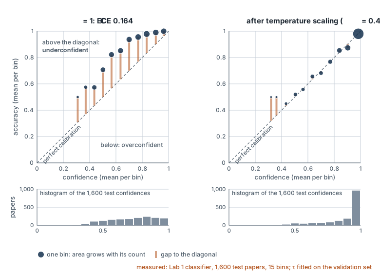
Two reliability diagrams for the Lab 1 classifier. Before temperature scaling the bins lie above the diagonal, meaning the model is right more often than its confidence says; after temperature scaling they lie on the diagonal. — Figure 1: Reliability diagrams of the Lab 1 classifier with `C = 1` on the 1,600 test papers, with M = 15 bins (Equation 2). Each dot is a non-empty bin, its area growing with the bin’s count, and the bar joining it to the diagonal is the bin’s gap. Left: the bins lie above the diagonal, so the model is right more often than its confidence says (underconfident); ECE 0.164 (Equation 3). Right: after temperature scaling with \tau^* = 0.47, fitted on the validation set (section 6), the bins lie on the diagonal; ECE 0.009. The confidences also move up: 962 of the 1,600 land in the top bin. The two lowest bins on the right hold 2 and 4 papers, so their gaps are noise. Recomputed with Lab 11’s code; data: `images/11-calibration.json`.

Expected calibration error. Summarize the diagram by the gaps, weighted by how many examples each bin holds (Naeini, Cooper and Hauskrecht, 2015):

\mathrm{ECE} = \sum_{m=1}^{M} \frac{\lvert B_m \rvert}{N}\, \big\lvert \mathrm{acc}(B_m) - \mathrm{conf}(B_m) \big\rvert . \tag{3}

ECE is 0 for a calibrated model in the limit of infinite data, and at most 1. Guo et al. (2017) used M = 15, and so do we. For the three classifiers of section 2 it is 0.164 (C = 1), 0.023 (C = 10) and 0.044 (C = 100).

Worked example: ECE on ten predictions in two bins. Take N = 10 predictions of a four-class model and M = 2 bins, (0, 0.5] and (0.5, 1].

Bin	Confidences \hat{p}	Outcomes o	\mathrm{conf}(B_m)	\mathrm{acc}(B_m)	Gap
B_1 = (0, 0.5]	0.3, 0.4, 0.4, 0.5	1, 0, 1, 0	1.6 / 4 = 0.40	2 / 4 = 0.50	0.10
B_2 = (0.5, 1]	0.6, 0.7, 0.8, 0.9, 0.9, 0.9	1, 1, 0, 1, 0, 1	4.8 / 6 = 0.80	4 / 6 = 0.67	0.13

By Equation 3, \mathrm{ECE} = \tfrac{4}{10} \times 0.10 + \tfrac{6}{10} \times 0.13 = 0.04 + 0.08 = 0.12. The low bin sits above the diagonal (underconfident) and the high bin below it (overconfident). The absolute value in Equation 3 stops the two from canceling. The confidence 0.5 goes in B_1 because the bins are closed on the right.

Five pitfalls. ECE is the most reported calibration number and one of the easiest to misread (Nixon et al., 2019).

It depends on M. For the C = 10 classifier on the same predictions: 0.022 with 5 bins, 0.023 with 15, 0.038 with 50, 0.055 with 100. Compare ECEs only at the same M, and report M.
It is positive for a perfectly calibrated model. With few examples per bin, \mathrm{acc}(B_m) is a noisy estimate and its absolute gap from \mathrm{conf}(B_m) is positive on average. We simulated a forecaster that is calibrated by construction (outcomes drawn with probability equal to the confidences of the C = 10 classifier). Its mean ECE at M = 15 was 0.074 on 100 examples, 0.043 on 300, and 0.019 on 1,600. So the C = 10 classifier’s 0.023 on 1,600 papers is within noise of perfect. Report N, and compare against this noise floor.
Equal-width bins crowd at the top. An accurate model puts most predictions above 0.9, so a few bins carry nearly all the weight and the rest are empty or nearly so. Equal-mass (adaptive) bins, each holding N/M examples, spread the estimate more evenly. The lab prints both.
Zero ECE does not mean a good model. The input-blind model of section 2 has ECE exactly 0. ECE says nothing about sharpness, and it is not a proper scoring rule (section 4): a model can lower it without becoming more useful. Report it next to a proper score.
It sees only the top class. Errors in how the remaining probability is spread over the other classes are invisible to it. The Brier score and the log loss of section 4 see the whole vector.

Check yourself. Recompute the ECE of the worked example with a single bin, M = 1. Which pitfall does the change illustrate, and is the smaller number better news about the model?

Answer

With one bin, \mathrm{conf} = 6.4/10 = 0.64 and \mathrm{acc} = 6/10 = 0.60, so \mathrm{ECE} = 0.04, a third of the two-bin value. Nothing about the model changed, so it is not better news: this is pitfall 1, the dependence on M. Inside the single bin the underconfident and the overconfident predictions cancel, as they did in section 2’s question. Fewer bins hide more; more bins leave fewer examples in each and raise the noise floor (pitfall 2). Report M and N with every ECE.

In the lab. In Exercise 1 you write reliability_bins(conf, correct, n_bins=15, adaptive=False), which returns the counts, mean confidences and accuracies of Equation 2, and ece(conf, correct, n_bins=15, adaptive=False), which is Equation 3. Checkpoints: a hand-made ten-example case with a known answer; ECE 0 for the input-blind model; ECE near 0 for a large synthetic set that is calibrated by construction. You then draw the reliability diagram of the classifier and print its ECE beside the simulated noise floor for the same N.

4. Proper Scoring Rules

In this section: define a proper scoring rule, prove that the Brier score is one, and say why accuracy is not.

ECE measures one property. We would also like a single score that a model can only improve by being both calibrated and sharp, and that cannot be gamed. That is what a proper scoring rule is.

Scoring rules. A scoring rule S(q, y) assigns a penalty to a reported distribution q once the label y is known. Two are standard. The Brier score (Brier, 1950) is the squared distance between the reported distribution and the one-hot label:

S_{\text{Brier}}(q, y) = \sum_{c=1}^{C} \big(q_c - \mathbf{1}[y = c]\big)^2 = \big\lVert q - \mathrm{onehot}(y) \big\rVert_2^2 . \tag{4}

It lies between 0 (all probability on the right class) and 2 (all on a wrong one). The log loss is the negative log-probability of the label:

S_{\text{log}}(q, y) = -\log q_y . \tag{5}

You know it already: averaged over a dataset with q = \hat{y}, it is Module 1’s cross-entropy loss, the quantity every classifier in this workshop was trained to minimize. Here we evaluate it on held-out data. In both cases the reported number is the average over the N evaluation examples, with q = \hat{y}^{(i)} and y = y^{(i)}.

Proper and strictly proper. Suppose the label is really drawn from a distribution p. A forecaster who reports q expects the penalty \mathbb{E}_{y \sim p}[S(q, y)]. The rule is proper if reporting the truth is never worse than any other report:

\mathbb{E}_{y \sim p}\big[S(p, y)\big] \;\le\; \mathbb{E}_{y \sim p}\big[S(q, y)\big] \qquad \text{for all } p, q \in \Delta^{C}, \tag{6}

and strictly proper if equality holds only at q = p (Gneiting and Raftery, 2007). Under a strictly proper rule, the unique way to minimize your expected penalty is to report what you believe. Exaggerating or hedging always costs.

The Brier score is strictly proper: a proof sketch. Write p_c = P(y = c) and expand one term of Equation 4. Since \mathbf{1}[y = c]^2 = \mathbf{1}[y = c] and its expectation is p_c,

\mathbb{E}_{y \sim p}\big[(q_c - \mathbf{1}[y = c])^2\big] = q_c^2 - 2 q_c p_c + p_c = (q_c - p_c)^2 + p_c (1 - p_c).

Summing over c:

\mathbb{E}_{y \sim p}\big[S_{\text{Brier}}(q, y)\big] = \underbrace{\sum_{c} (q_c - p_c)^2}_{\text{depends on the report}} \;+\; \underbrace{\sum_{c} p_c (1 - p_c)}_{\text{does not}} . \tag{7}

The second term is fixed by the world. The first is a squared distance, zero exactly when q = p and positive otherwise. So the expected Brier score is minimized by q = p and by nothing else, which is Equation 6 with strict inequality.

The log loss is strictly proper too. Its expectation is -\sum_c p_c \log q_c, the cross-entropy of q on data from p. Module 10 used the identity that this equals the entropy of p plus \mathrm{KL}(p \,\Vert\, q). The entropy does not depend on q, and the KL divergence is zero only at q = p. The log loss punishes confident mistakes without limit (-\log q_y \to \infty as q_y \to 0), so one overconfident error can dominate an average; the Brier score is bounded. Report both.

Accuracy is not strictly proper. Treat accuracy as a penalty, S_{\text{acc}}(q, y) = \mathbf{1}[\arg\max_c q_c \neq y]. Its expectation is 1 - p_{\arg\max q}: it depends on q only through which class is largest. Reporting 0.51 or 0.99 for the same class earns exactly the same expected score. Accuracy is proper in the weak sense, because the truth is among the best reports, but it gives no reason to report the truth rather than any distribution with the same top class. A model selected by accuracy alone has no pressure to be calibrated.

Some plausible scores are improper. The linear score, S_{\text{lin}}(q, y) = -q_y (“reward the probability given to the right answer”), looks reasonable. Its expectation is -\sum_c p_c q_c, which is minimized by putting all the probability on the most likely class. It rewards overconfidence. If the true distribution is (0.7, 0.3), the linear score prefers the report (1, 0); the Brier score and the log loss prefer (0.7, 0.3); accuracy cannot tell any report with q_1 > 0.5 from another.

Why this matters beyond evaluation. Training a model is choosing a scoring rule to minimize. Cross-entropy is strictly proper, so at its optimum over all possible predictors, on the true data distribution, it gives calibrated probabilities. The words “over all predictors” and “on the true distribution” carry the weight: a real model minimizes it on a finite training set, with a restricted function class. Section 5 is about what happens in between. And training against something that is not a proper score, such as a preference between two answers (Module 10), gives no such guarantee at all.

Score	Range	Strictly proper	Sees the whole \hat{y}	`C = 1`	`C = 10`	`C = 100`
ECE (M = 15)	0 to 1	no (not a scoring rule)	no	0.164	0.023	0.044
Brier score, Equation 4	0 to 2	yes	yes	0.211	0.166	0.176
Log loss, Equation 5	0 to \infty	yes	no, only \hat{y}_y	0.436	0.314	0.339
Error rate (1 - accuracy)	0 to 1	no	no	0.113	0.116	0.118

Measured on the 1,600 test papers, as in section 2. The proper scores rank C = 10 first; the error rate ranks it second.

Optional: The Brier Score’s Three Parts

Murphy (1973) split the average Brier score into three terms. For one binary event (for example “the prediction is correct”, with forecast \hat{p}), with forecasts grouped into bins B_m and overall base rate \bar{o}:

\frac{1}{N} \sum_{i} \big(\hat{p}^{(i)} - o^{(i)}\big)^2 \approx \underbrace{\sum_{m} \tfrac{\lvert B_m \rvert}{N} \big(\mathrm{conf}(B_m) - \mathrm{acc}(B_m)\big)^2}_{\text{reliability (miscalibration)}} - \underbrace{\sum_{m} \tfrac{\lvert B_m \rvert}{N} \big(\mathrm{acc}(B_m) - \bar{o}\big)^2}_{\text{resolution (sharpness that pays)}} + \underbrace{\bar{o}\,(1 - \bar{o})}_{\text{uncertainty}} .

The approximation is exact when every forecast in a bin is the same. The first term is a squared version of ECE’s gap; the second rewards bins whose accuracy differs from the base rate; the third is fixed by the data. One proper score contains the two goals of section 2: calibration and sharpness.

Check yourself. The label of a two-class item is drawn from p = (0.7, 0.3). Use Equation 7 to compute the expected Brier score of three reports: the honest (0.7, 0.3), the exaggerated (1, 0) and the hedged (0.5, 0.5). Then rank the same three by expected log loss. Do the two rules agree on which dishonest report is worse?

Answer

The fixed term is \sum_c p_c(1 - p_c) = 0.21 + 0.21 = 0.42. The report-dependent term is 0 for the honest report, 0.3^2 + 0.3^2 = 0.18 for (1, 0) and 0.2^2 + 0.2^2 = 0.08 for (0.5, 0.5). So the expected Brier scores are 0.42, 0.60 and 0.50. The expected log loss is -(0.7 \log 0.7 + 0.3 \log 0.3) = 0.611 for the honest report, \log 2 = 0.693 for the hedge, and infinite for (1, 0), because 30% of the time it gave the label probability zero. Both rules put honesty first and the exaggeration last. They differ in how hard they punish it: the Brier score by a bounded 0.18, the log loss without limit.

In the lab. In Exercise 2 you write brier(probs, labels) (Equation 4) and nll(probs, labels) (Equation 5), each averaged over examples. Checkpoints: hand computations on three examples; the uniform four-class model scores exactly 0.75 and \log 4; nll agrees with sklearn.metrics.log_loss. A provided cell then prints the table above for your classifier and for the three Lab 1 models. The stretch section shows numerically that the expected Brier score is minimized by the true probability (Equation 7), that the linear score is not, and that accuracy is flat.

5. Why Models Are Miscalibrated

In this section: give the known reasons that trained networks and preference-tuned language models are often miscalibrated, and say which claims are settled.

Classifiers. Guo et al. (2017) compared older and newer networks for image and text classification and found the newer, deeper and wider ones markedly overconfident, where older, smaller networks such as LeNet had been close to calibrated. Depth, width, batch normalization and weaker weight decay all moved models toward overconfidence. Their explanation is overfitting in the log loss. Once a network classifies almost every training example correctly, it can still lower its training cross-entropy by making every correct prediction more confident, which it does by growing the logits. On held-out data the classification error stays put while the confidence keeps rising; held-out log loss gets worse before held-out accuracy does.

Our linear classifier shows the same lever on a small scale. In section 2, weakening the L2 penalty (larger C) let the weights, and so the logits, grow, and moved the model from underconfident to overconfident while its accuracy barely changed.

Three qualifications, all from later measurements.

Not every modern network. Minderer et al. (2021) found that recent architectures that do not use convolutions, such as vision transformers, were among the best calibrated models they tested, and that architecture mattered more than model size or the amount of pretraining.
Fine-tuned pretrained transformers in particular. Desai and Durrett (2020) found BERT and RoBERTa, fine-tuned for language-understanding tasks, relatively well calibrated in-domain, with temperature scaling reducing the error further, and worse calibrated out of domain. So we do not know in advance which way the Lab 6 encoder will fall. You will measure it.
Calibration does not survive a change of data. Ovadia et al. (2019) found that calibration measured on in-distribution data, including after post-hoc fixes like the one in section 6, degraded under dataset shift. A model calibrated on 2024 arXiv abstracts is not thereby calibrated on 2027 ones.

Language models. Two kinds of evidence point in the same direction for preference-tuned models.

Pretrained models can be calibrated on the right format. Kadavath et al. (2022) found that large pretrained language models were well calibrated on multiple-choice and true/false questions when the options were presented in a suitable format, reading the confidence from the probability given to each answer’s letter.
Post-training has reduced that calibration in reported cases. The GPT-4 technical report (OpenAI, 2023) shows the pretrained model’s answer probabilities on a subset of the MMLU benchmark lying close to the diagonal of a reliability diagram, and the model after post-training with PPO lying well off it. Tian et al. (2023) likewise found the token probabilities of several RLHF-tuned models (ChatGPT, GPT-4 and Claude among them) poorly calibrated on question-answering benchmarks.

Why would preference training do this? Module 10 gives two reasons to expect it, neither of which is a measured mechanism: the reward compares whole answers and never rewards an appropriate hedge, and the optimum of the KL-regularized objective, \pi^* \propto \pi_{\text{ref}}\, e^{r/\beta}, moves probability toward the responses the reward rates highest, which sharpens the distribution over answers. What is established is the measured effect in the reported cases. How general it is, and which part of post-training causes it, are open questions.

The practical conclusion. Never assume a model is calibrated, in either direction. Measure it, on data like the data it will see, and recheck when the data change.

Check yourself. You train a network for five more epochs. Its held-out accuracy does not move, and its held-out log loss rises. What happened to its confidences, what does its reliability diagram look like now, and which way would a fitted temperature move from 1?

Answer

The predictions did not change, so the probabilities did: the logits grew and every prediction became more confident. On the held-out examples the model gets right, the log loss can fall only a little, because those probabilities were already near 1. On the ones it gets wrong, the probability of the true class shrinks and -\log \hat{y}_y grows without limit, so the average rises. The reliability diagram’s points move right at the same accuracy, below the diagonal: overconfidence. A fitted temperature would come out above 1 (section 6). This is Guo et al.’s overfitting in the log loss.

6. Temperature Scaling

In this section: fit one number that recalibrates a classifier without changing its predictions, and say what it cannot fix.

Why a fix is needed. Section 5, for reading after class, collects the evidence on why trained models are miscalibrated. In short: a network that already gets its training examples right can keep lowering its training log loss by growing its logits, which makes it overconfident on new data (Guo et al., 2017). The three classifiers of section 2 show the same lever: a weaker penalty on the weights let the logits grow and turned underconfidence into overconfidence. Not every architecture goes that way, calibration does not survive a change of data, and preference-tuned language models have lost the calibration of their token probabilities in reported cases. Never assume a model is calibrated: measure it.

The fix. Divide the logits by a temperature \tau > 0 before the softmax:

\hat{y}(\tau) = \mathrm{softmax}\big(z / \tau\big). \tag{8}

This is the operation of Module 3’s temperature sampling, used for a different purpose. There, \tau was chosen to make samples more or less varied. Here it is fitted, once, to make the probabilities honest. \tau > 1 flattens \hat{y} and fixes overconfidence; \tau < 1 sharpens it and fixes underconfidence.

The fit. Choose \tau to minimize the log loss on the validation set, with the model’s weights frozen:

\tau^* = \arg\min_{\tau > 0}\; -\frac{1}{N_{\text{val}}} \sum_{i=1}^{N_{\text{val}}} \log \mathrm{softmax}\big(z^{(i)} / \tau\big)_{y^{(i)}} , \tag{9}

where N_{\text{val}} is the number of validation examples. Then report every metric on the test set with \tau^* fixed. Fitting on test would report a calibration that no deployed model could have.

Four properties. Each one is a reason the method is the standard first step (Guo et al., 2017).

It does not change any prediction. Dividing all logits by the same positive number keeps their order, so \hat{c} is unchanged for every example, and accuracy is exactly the same. Module 3 said it: temperature changes the sharpness of a distribution, never its ranking.
It fits a proper score. The objective is the log loss, which is strictly proper (section 4), smooth, and needs no bins. Fitting \tau to ECE instead would inherit every pitfall of section 3.
It has one parameter. One number cannot overfit 600 validation papers.
The fit is a one-dimensional convex problem in 1/\tau (optional box below), so a bracketing search, or Newton’s method, finds the global minimum.

Optional: Why the Temperature Fit Is Convex

Write \beta = 1/\tau. For one example the loss is -\beta z_y + \log \sum_c e^{\beta z_c}: a linear function of \beta plus a log-sum-exp of linear functions of \beta, which is convex. Its derivative is \sum_c \hat{y}_c(\tau)\, z_c - z_y, the model’s expected logit minus the logit of the correct class. A bracketing search over \beta, or Newton’s method, finds the global minimum.

from scipy.optimize import minimize_scalar
from scipy.special import log_softmax

def fit_temperature(val_logits, val_labels):
    """val_logits: (N, C) raw logits; val_labels: (N,) ints. Returns tau > 0."""
    rows = np.arange(len(val_labels))
    def val_nll(log_tau):                         # search over log tau: tau stays positive
        logp = log_softmax(val_logits / np.exp(log_tau), axis=1)
        return -logp[rows, val_labels].mean()     # the log loss of eq-temp-fit
    return float(np.exp(minimize_scalar(val_nll, bounds=(-3, 3), method="bounded").x))

Measured, on the three Lab 1 classifiers (fitted on the 600 validation papers, evaluated on the 1,600 test papers, build container, 2026-10-05):

`C`	\tau^*	Accuracy before → after	ECE before → after	Log loss before → after	Brier before → after
1	0.47	0.888 → 0.888	0.164 → 0.009	0.436 → 0.303	0.211 → 0.164
10	0.79	0.884 → 0.884	0.023 → 0.018	0.314 → 0.307	0.166 → 0.165
100	1.30	0.882 → 0.882	0.044 → 0.017	0.339 → 0.319	0.176 → 0.171

The direction of \tau^* matches the reading of section 2: below 1 for the underconfident model, above 1 for the overconfident one. After scaling, all three ECEs sit within the noise floor of section 3 for 1,600 examples. The C = 10 model, already calibrated within noise, barely moves.

What it cannot fix.

Errors that differ across inputs. One \tau rescales every example alike. A model overconfident on robotics papers and underconfident on language papers keeps both errors in a different mix.
A change of data. \tau^* is fitted to the validation distribution (section 5, Ovadia et al.).
A model without logits. The commercial models of Module 8 do not give you full logits over their answers, and a confidence written in words has none. Section 7 measures such a confidence instead, and other recalibration maps that need only a confidence and an outcome, listed below, still apply.

Optional: Other Post-Hoc Calibration Maps

All of these are fitted on validation data and leave the model’s weights alone.

Platt scaling (Platt, 1999) fits a logistic regression from a binary classifier’s score to the label. Temperature scaling is its one-parameter multiclass version: a single slope, no intercept, shared by all classes.
Histogram binning replaces each confidence by the validation accuracy of its bin; isotonic regression (Zadrozny and Elkan, 2002) fits the best non-decreasing map from confidence to accuracy. Both are more flexible than temperature scaling and need more validation data; neither is guaranteed to preserve the ranking of examples with tied outputs.
Vector and matrix scaling (Guo et al., 2017) fit a separate scale per class, or a full linear map of the logits. Guo et al. found that they overfit more easily and did not beat temperature scaling on most of their datasets.

Niculescu-Mizil and Caruana (2005) compare Platt scaling and isotonic regression across many classical models.

Demo: one temperature moves the whole reliability diagram. The 4,000 synthetic four-class predictions below come from a model that is overconfident by construction: each label was drawn from \mathrm{softmax}(z^\ast) for random logits z^\ast, and the model reports z = 2.5\, z^\ast. The slider sets \tau in Equation 8. Predict first. Which \tau puts the points on the diagonal, and what happens to the accuracy on the way there?

viewof tau11 = Inputs.range([0.5, 5], {value: 1, step: 0.05, label: "temperature τ"})

toy11 = {
  let s = 11;                                    // fixed seed: the same 4,000 examples on every load
  const rand = () => { s = (s + 0x6D2B79F5) | 0; let t = Math.imul(s ^ (s >>> 15), 1 | s);
    t = (t + Math.imul(t ^ (t >>> 7), 61 | t)) ^ t; return ((t ^ (t >>> 14)) >>> 0) / 4294967296; };
  const gauss = () => Math.sqrt(-2 * Math.log(1 - rand())) * Math.cos(2 * Math.PI * rand());
  const softmax = z => { const m = Math.max(...z), e = z.map(v => Math.exp(v - m)), t = e.reduce((a, b) => a + b);
    return e.map(v => v / t); };
  const data = Array.from({length: 4000}, () => {
    const zs = Array.from({length: 4}, () => 1.5 * gauss()), p = softmax(zs);
    let u = rand(), y = 0; while (y < 3 && u > p[y]) { u -= p[y]; y++; }     // y ~ softmax(z*)
    return {z: zs.map(v => 2.5 * v), y};                                     // reported logits
  });
  const metrics = tau => {                       // eq-temp-scaling, eq-bin-stats, eq-ece (M = 15), eq-log-loss
    const M = 15, bins = Array.from({length: M}, () => ({n: 0, conf: 0, acc: 0}));
    let nll = 0, hits = 0;
    for (const {z, y} of data) {
      const p = softmax(z.map(v => v / tau)), conf = Math.max(...p), hit = p.indexOf(conf) === y ? 1 : 0;
      const b = bins[Math.min(M - 1, Math.max(0, Math.ceil(conf * M) - 1))];
      b.n++; b.conf += conf; b.acc += hit; nll -= Math.log(p[y]); hits += hit;
    }
    const N = data.length, pts = bins.filter(b => b.n).map(b => ({conf: b.conf / b.n, acc: b.acc / b.n, n: b.n}));
    return {tau, pts, nll: nll / N, acc: hits / N, ece: pts.reduce((a, b) => a + b.n / N * Math.abs(b.acc - b.conf), 0)};
  };
  return {metrics, curve: Array.from({length: 46}, (_, i) => metrics(0.5 + 0.1 * i))};
}

{
  const m = toy11.metrics(tau11), ink = "currentColor", navy = "var(--demo-blue)", warm = "var(--demo-orange)";
  const left = Plot.plot({width: 360, height: 340, grid: true,
    x: {domain: [0, 1], label: "confidence (mean per bin)"}, y: {domain: [0, 1], label: "accuracy (mean per bin)"},
    r: {range: [2, 9]},
    marks: [Plot.line([[0, 0], [1, 1]], {stroke: ink, strokeDasharray: "4 4"}),
      Plot.link(m.pts, {x1: "conf", x2: "conf", y1: "conf", y2: "acc", stroke: warm, strokeWidth: 2}),
      Plot.dot(m.pts, {x: "conf", y: "acc", r: "n", fill: navy})]});
  const right = Plot.plot({width: 360, height: 340, grid: true,
    x: {label: "temperature τ"}, y: {domain: [0, 1.6], label: "value on the 4,000 examples"},
    marks: [Plot.line(toy11.curve, {x: "tau", y: "nll", stroke: navy}), Plot.line(toy11.curve, {x: "tau", y: "ece", stroke: warm}),
      Plot.ruleX([tau11], {stroke: ink, strokeDasharray: "2 3"}),
      Plot.dot([m], {x: "tau", y: "nll", fill: navy, r: 4}), Plot.dot([m], {x: "tau", y: "ece", fill: warm, r: 4}),
      Plot.text([{x: 4.9, y: toy11.curve[44].nll + 0.07, t: "log loss"}], {x: "x", y: "y", text: "t", fill: navy, textAnchor: "end"}),
      Plot.text([{x: 4.9, y: toy11.curve[44].ece + 0.07, t: "ECE (M = 15)"}], {x: "x", y: "y", text: "t", fill: warm, textAnchor: "end"})]});
  return html`<div style="display:flex;gap:1rem;flex-wrap:wrap">${left}${right}</div>
    <p><strong>τ = ${tau11.toFixed(2)}</strong>: accuracy ${m.acc.toFixed(3)}, ECE ${m.ece.toFixed(3)}, log loss ${m.nll.toFixed(3)}</p>`;
}

What it shows. Left: the reliability diagram at the chosen \tau, one dot per non-empty bin of Equation 2, sized by its count, with its gap to the diagonal drawn. Right: the log loss (Equation 5) and ECE (Equation 3) of the same predictions against \tau. At \tau = 1 the dots hang below the diagonal, further the higher the confidence. Near \tau = 2.5, the factor the logits were inflated by, the dots reach the diagonal and both curves reach their minimum; past it the model turns underconfident and both rise again. The accuracy never changes (property 1). The log-loss curve is smooth with a single minimum, which is why Equation 9 fits \tau to it and not to ECE. The data are synthetic and say nothing about any real model. Both curves are drawn on one set of examples; a real fit chooses \tau on validation data and reports on test data.

Check yourself. One example has logits z = (2, 1, 0). Compute its confidence \hat{p} at \tau = 1 and at \tau = 2. A colleague then proposes to fit \tau by maximizing validation accuracy. What will that search find?

Answer

At \tau = 1: \hat{p} = e^2 / (e^2 + e^1 + e^0) = 0.665. At \tau = 2 the logits become (1, 0.5, 0) and \hat{p} = e^1 / (e^1 + e^{0.5} + e^0) = 0.506. The predicted class is the first one both times, because dividing by a positive number keeps the order of the logits. For the same reason validation accuracy is the same for every \tau > 0: the colleague’s objective is flat, and the search returns an arbitrary value. Accuracy cannot tell 0.665 from 0.506 (section 4), so it cannot fit a parameter that changes only the confidence. The log loss can.

In the lab. In Exercise 3 you write fit_temperature(val_logits, val_labels) (Equation 8, Equation 9). Checkpoints: on synthetic logits from a calibrated model multiplied by 3, it recovers \tau \approx 3; the validation log loss at \tau^* is no higher than at \tau = 1; test accuracy is identical before and after. You then print the before-and-after table for your classifier and for the three Lab 1 models, and draw the reliability diagrams side by side.

7. Confidence From a Language Model Behind an API

In this section: obtain a confidence from a model you cannot inspect, and measure it with the tools of sections 3 and 4.

A language model reached through an API returns text. Three sources of confidence are available, depending on access.

Source	How	Needs
Answer-token probability	the probability the model gives to the token of each allowed answer (`yes` or `no`, an option letter), renormalized over the options	the model’s logits: a local model, or a provider that returns log-probabilities for your model
Verbalized confidence	ask for the answer and “the probability, between 0 and 1, that your answer is correct” in the same structured reply	nothing beyond the API
Consistency	sample several answers to the same question; the confidence is the share that agree with the most common one	several calls per question

What is known about verbalized confidence. It can be learned; for preference-tuned models it is sometimes better calibrated than the token probabilities; and out of the box it tends to be overconfident and coarse. The optional box below gives the studies.

Optional: The Studies Behind These Three Findings

It can be learned. Lin, Hilton and Evans (2022) fine-tuned GPT-3 to state a confidence with its answer, and the stated confidences were well calibrated on arithmetic questions, including under some distribution shift.
For preference-tuned models it can beat the token probabilities. Tian et al. (2023) found that for several RLHF-tuned models, confidences stated as output tokens were often better calibrated than the models’ own token probabilities, on TriviaQA, SciQ and TruthfulQA.
Out of the box it tends to be overconfident and coarse. Xiong et al. (2024) found stated confidences concentrated between 80% and 100%, mostly in multiples of 5, as people tend to state them, and found no elicitation method that was best across tasks.

So a stated confidence is neither worthless nor trustworthy. It is one more output of the model, and like the extraction of Module 8 it has to be evaluated on labeled data. The measurements are the ones you have already: treat the stated number as \hat{p}, the answer as \hat{c}, and compute the reliability diagram, ECE, the Brier score and the log loss of the binary event “the answer is correct”.

The protocol. The lab reuses Module 8’s machinery: the provider wrapper, the PROVIDER switch, and validate-and-retry against a schema with two fields, the answer (restricted to the item’s options) and the confidence. The range 0 \le \hat{p} \le 1 is checked by your validator, not by the provider: Module 8 noted that Anthropic’s structured outputs do not support numeric ranges. When you read the result, keep in mind that stated confidences are coarse, that the prompt is part of the measurement, and that a few hundred questions give a noisy ECE; the optional box below says what each one means for the lab’s numbers.

Optional: Three Things to Keep in Mind When Reading the Result

Coarse values make ties. If every stated confidence is 0.9 or 0.95, most bins are empty, and the ranking of section 8 has large flat steps.
The prompt is part of the measurement. Asking for the answer before or after the confidence, or in words (“high”, “low”) rather than numbers, changes what comes back. The lab fixes one prompt and prints it; change it and you have a different measurement.
Small evaluation sets are noisy. On 300 questions, the noise floor of a perfectly calibrated forecaster’s ECE is about 0.04 (section 3). A difference of 0.02 between two providers on that set is not a finding.

The decision set. Calibration needs labels that are true, not preferred. The lab uses a small workshop-built set of decisions an assistant for a workshop’s front desk must make: is a cancellation eligible for a full refund under the written policy, should a request be routed to a calculator, a document lookup, an email, a question back to the user, or a human. Every label follows from a written policy, so it can be checked. Labs 12 and 14 reuse the same set. The lab prints three items and the start and end of the policy prompt before you start; how the set was built and labeled is recorded with the data.

In the lab. In Exercise 4 you write parse_decision(reply_text, options), which turns a reply into an answer and a confidence, or None if either is missing or out of range. The checkpoint runs it on recorded reply strings and is the same on every provider. A provided loop then asks the model selected by PROVIDER for an answer and a confidence on each item of the decision set, and your functions from Exercises 1 and 2 report its accuracy, ECE, Brier score and reliability diagram, with a histogram of the stated confidences. On the open model the lab also reads the answer-token probability and compares the two. No model’s calibration is asserted. If no model can be reached, the lab runs on a stub that writes replies in the same format; it exercises your code, and its numbers are labeled as a test double and are not a measurement of anything.

Check yourself. A language model answers 300 questions and states a confidence with each. It says 0.9 on 200 of them, of which 150 are right, and 0.95 on the other 100, of which 90 are right. With M = 15 equal-width bins, how many bins are non-empty, and what is the ECE? Is the result within the noise floor of a calibrated forecaster on 300 questions?

Answer

Two bins: 0.9 falls in (13/15, 14/15] and 0.95 in (14/15, 1]. Their accuracies are 150/200 = 0.75 and 90/100 = 0.90, so the gaps are 0.15 and 0.05, and \mathrm{ECE} = \tfrac{200}{300} \times 0.15 + \tfrac{100}{300} \times 0.05 = 0.117. That is about three times the noise floor of 0.04 quoted above for 300 questions, so this model is overconfident beyond what chance explains: it claims 0.917 on average and is right 80% of the time. The stated confidences still carry some information, since the 0.95 group is right more often than the 0.9 group. With only two distinct values, though, the risk–coverage curve of section 8 has only two steps.

8. Selective Prediction and the Cost of a Wrong Action

In this section: turn a confidence into a decision to act or defer, and choose the threshold from a stated cost.

Selective prediction. A system may abstain: decline to act on a prediction and pass the case to a person. With a threshold \lambda, it acts when \hat{p} \ge \lambda and defers otherwise. Two numbers describe the result on a set of N examples:

\mathrm{coverage}(\lambda) = \frac{1}{N} \sum_{i=1}^{N} \mathbf{1}\big[\hat{p}^{(i)} \ge \lambda\big], \qquad \mathrm{risk}(\lambda) = \frac{\sum_{i} \mathbf{1}\big[\hat{p}^{(i)} \ge \lambda\big]\,\big(1 - o^{(i)}\big)}{\sum_{i} \mathbf{1}\big[\hat{p}^{(i)} \ge \lambda\big]} . \tag{10}

Coverage is the share of cases the system handles; selective risk is the error rate among them. Sweeping \lambda from 1 down to 0 traces the risk–coverage curve (El-Yaniv and Wiener, 2010; Geifman and El-Yaniv, 2017), from “act on nothing” to “act on everything”, where the risk is the plain error rate.

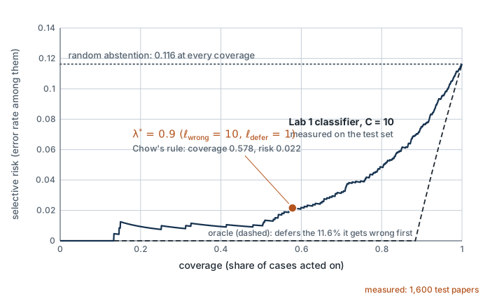
Risk–coverage curve of the Lab 1 classifier. Acting only on its most confident predictions lowers the error rate from 11.6 percent at full coverage to about 2 percent at 58 percent coverage, between the random-abstention line and the oracle. — Figure 2: Risk–coverage curve (Equation 10) of the Lab 1 classifier with `C = 10` on the 1,600 test papers, acting on its most confident predictions first. At full coverage the risk is the plain error rate, 0.116, and random abstention keeps it there at every coverage. The oracle, which knows which predictions are wrong, defers those first. Chow’s rule with \ell_{\text{wrong}} = 10 and \ell_{\text{defer}} = 1 gives \lambda^* = 0.9 (Equation 11): coverage 0.578, risk 0.022. Recomputed with Lab 11’s code; data: `images/11-calibration.json`.

Ranking, not calibration, sets the curve. The curve depends only on the order of the confidences: which cases are handled first. Any increasing transformation of \hat{p} leaves it unchanged. Temperature scaling is one for two classes, but not exactly for more: rescaling all the logits can reorder the top-class probabilities of two examples. In Lab 11’s four-class classifier it swapped the order of 0.92% of test pairs and moved the area under the curve from 0.0274 to 0.0268, a small change. A good curve needs a confidence that ranks errors last. Calibration matters for the next step: choosing where on the curve to stand.

The threshold from a cost. Let acting on a correct prediction cost nothing, acting on a wrong one cost \ell_{\text{wrong}}, and deferring cost \ell_{\text{defer}} (a person’s time), with \ell_{\text{defer}} < \ell_{\text{wrong}}. If the confidence is calibrated, a prediction with confidence \hat{p} is wrong with probability 1 - \hat{p}, so the expected cost of acting is (1 - \hat{p})\, \ell_{\text{wrong}} and that of deferring is \ell_{\text{defer}}. Act when acting is cheaper:

(1 - \hat{p})\, \ell_{\text{wrong}} < \ell_{\text{defer}} \quad\Longleftrightarrow\quad \hat{p} > \lambda^* = 1 - \frac{\ell_{\text{defer}}}{\ell_{\text{wrong}}} . \tag{11}

(At \hat{p} = \lambda^* the two costs are equal and either choice will do; the lab acts.) This is Chow’s rule (Chow, 1970). A wrong action ten times as costly as a review gives \lambda^* = 0.9; twenty times, 0.95. The threshold is set by the costs, not by a habit such as “0.5” or “0.8”, and it is only as good as the calibration: an overconfident model passes the threshold on cases it gets wrong more often than 1 - \lambda^*.

The threshold from data. Without trusting calibration, choose \lambda to minimize the average cost on the validation set directly:

\widehat{\mathrm{cost}}(\lambda) = \frac{1}{N} \sum_{i=1}^{N} \Big( \mathbf{1}\big[\hat{p}^{(i)} \ge \lambda\big]\,\big(1 - o^{(i)}\big)\, \ell_{\text{wrong}} + \mathbf{1}\big[\hat{p}^{(i)} < \lambda\big]\, \ell_{\text{defer}} \Big) = \mathrm{coverage}(\lambda)\, \mathrm{risk}(\lambda)\, \ell_{\text{wrong}} + \big(1 - \mathrm{coverage}(\lambda)\big)\, \ell_{\text{defer}} , \tag{12}

with N the number of validation examples here. Only values of \lambda equal to an observed confidence (plus 0 and a value above the largest) need to be tried. Then report the cost, coverage and risk on the test set at the chosen \lambda. With a calibrated model the two thresholds agree; a gap between them is a measurement of miscalibration where it matters, near the threshold.

Worked example: five predictions by hand. Sorted by confidence, five predictions have \hat{p} = 0.95, 0.9, 0.8, 0.7, 0.6 and outcomes o = 1, 1, 0, 1, 0. Take \ell_{\text{wrong}} = 10 and \ell_{\text{defer}} = 1.

Threshold \lambda	Acted on	Coverage	Risk (Equation 10)	Cost per case (Equation 12)
above 0.95	none	0	–	5 \times 1 / 5 = 1.0
0.95	1	0.2	0/1 = 0	(0 + 4)/5 = 0.8
0.9	2	0.4	0/2 = 0	(0 + 3)/5 = 0.6
0.8	3	0.6	1/3 = 0.33	(10 + 2)/5 = 2.4
0.7	4	0.8	1/4 = 0.25	(10 + 1)/5 = 2.2
0.6 or below	all 5	1.0	2/5 = 0.40	20/5 = 4.0

The cheapest threshold is \lambda = 0.9, at 0.6 per case, and Chow’s rule gives the same value, \lambda^* = 1 - 1/10 = 0.9. One wrong action costs as much as ten reviews, so the first error, admitted at \lambda = 0.8, outweighs everything gained by deferring less. Risk is not monotone in coverage: it falls from 0.33 to 0.25 when the fourth prediction, a correct one, is admitted.

On the measured C = 10 classifier, with the same costs, acting on everything costs more per case than sending everything to a person, and abstaining on the least confident 31 to 42% of cases halves the cost of either. The optional box below has the numbers, policy by policy.

Optional: The Measured Classifier, Policy by Policy

Worked example: the measured classifier (the C = 10 Lab 1 classifier, \ell_{\text{wrong}} = 10, \ell_{\text{defer}} = 1, test set, build container, 2026-10-05).

Policy	Coverage	Risk	Cost per case
act on everything (\lambda = 0)	1.000	0.116	1.16
defer everything	0	–	1.00
Chow’s rule, \lambda^* = 0.9 (Equation 11)	0.578	0.022	0.55
\lambda chosen on validation (Equation 12): 0.84	0.676	0.029	0.52
Chow’s rule after temperature scaling (\tau^* = 0.79)	0.693	0.030	0.51

Acting on everything costs more than sending everything to a person. Abstaining on the least confident 31 to 42% of cases halves the cost of either. Before temperature scaling this model is slightly underconfident at the top, so Chow’s rule abstains more than it needs to; after scaling, the rule and the empirical choice land close together, as they should for a calibrated model.

Towards Module 12. Two actions are rarely enough. An assistant might act, ask the user a clarifying question, or escalate to a person, each with its own cost; two thresholds then split the confidence range into three regions, and the same reasoning sets both. Module 12 does this with a decision model that returns probabilities with every typed answer, using the decision set of this lab.

Check yourself. A wrong action costs 50 and a review costs 2. What threshold does Chow’s rule give? You then find, on validation data, that predictions with \hat{p} at or above that threshold are right only 90% of the time. What does acting on them cost per case, and what should you do about it?

Answer

\lambda^* = 1 - 2/50 = 0.96. The rule assumes that a prediction above the threshold is wrong at most 4% of the time. Here it is wrong 10% of the time, so acting costs 0.10 \times 50 = 5 per case, against 2 for a review: on these cases the rule does worse than deferring. Chow’s rule is only as good as the calibration behind it. Either recalibrate first (section 6) and apply the rule to the repaired confidences, or choose \lambda directly on validation data with Equation 12, which uses the outcomes and trusts no probability.

In the lab. In Exercise 5 you write risk_coverage(conf, correct), which returns coverage and risk at every threshold (Equation 10), and choose_threshold(conf, correct, l_wrong, l_defer), which minimizes Equation 12. Checkpoints: a hand-made six-example case; risk at full coverage equals the error rate; the chosen threshold’s validation cost is no higher than acting on everything or deferring everything. You then draw the risk–coverage curves of the classifier and of the language model, print the test cost at your threshold beside Chow’s \lambda^*, and compare the classifier’s curve before and after temperature scaling: unchanged for two classes (asserted), slightly changed for four (printed).

Equations and Where You Implement Them

Equation	Lab 11
Calibration (Equation 1)	read off every reliability diagram in Exercises 1, 3 and 4
Bin statistics and ECE (Equation 2, Equation 3)	Exercise 1: `reliability_bins`, `ece`; the provided noise-floor simulation
Brier score and log loss (Equation 4, Equation 5)	Exercise 2: `brier`, `nll`
Proper scoring rules (Equation 6, Equation 7)	Stretch: expected scores against the reported probability
Temperature scaling and its fit (Equation 8, Equation 9)	Exercise 3: `fit_temperature`
Calibration of a verbalized confidence (section 7)	Exercise 4: `parse_decision`, then Exercises 1 and 2 on the decision set
Coverage and selective risk (Equation 10)	Exercise 5: `risk_coverage`
Chow’s threshold and the empirical cost (Equation 11, Equation 12)	Exercise 5: `choose_threshold`, with \lambda^* printed beside it
Murphy’s decomposition (optional callout)	not implemented

Summary

A confidence is calibrated when, among predictions made with confidence p, a fraction p are right (Equation 1). Calibration and accuracy are different properties: an input-blind model is calibrated, and three classifiers within 0.6 points of each other in accuracy differ by 20 points in mean confidence.
Reliability diagrams and ECE estimate calibration from binned examples (Equation 2, Equation 3). ECE depends on the number of bins, is positive for a perfectly calibrated model on finite data, crowds into the top bins, ignores sharpness and sees only the top class. Report M, N and the noise floor.
A strictly proper scoring rule is minimized in expectation only by the true distribution (Equation 6). The Brier score is strictly proper because its expectation is a squared distance to the truth plus a constant (Equation 7); the log loss is, because its expectation is entropy plus a KL divergence. Accuracy cannot tell 0.51 from 0.99, and the linear score rewards overconfidence.
Modern networks are often overconfident because they keep lowering the training log loss by growing their logits (Guo et al.), but not all are: architecture matters, fine-tuned pretrained transformers can be close to calibrated in-domain, and calibration degrades under shift. Preference-tuned language models have lost token-probability calibration in reported cases; the cause is not settled.
Temperature scaling divides the logits by one number fitted to the validation log loss (Equation 8, Equation 9). It never changes a prediction, and it cannot fix errors that differ across inputs or survive a change of data.
A language model’s stated confidence is an output to be measured like any other, with the same metrics, on labeled data. It is often coarse and overconfident, and sometimes better than the model’s token probabilities.
The risk–coverage curve depends only on the ranking of confidences (Equation 10). The threshold comes from the cost of a wrong action: \lambda^* = 1 - \ell_{\text{defer}} / \ell_{\text{wrong}} for a calibrated model (Equation 11), or the minimizer of the validation cost otherwise (Equation 12).

Gotchas and Troubleshooting

“A softmax output is a probability.” It is a vector of non-negative numbers that sum to 1. Whether it behaves like a probability is an empirical question about the model and the data, answered by measuring calibration.
“A more accurate model is better calibrated.” The two move independently (section 2). The Lab 1 classifiers with the best and worst accuracy are the two worst calibrated.
“Low ECE means a good model.” The input-blind model has ECE 0. ECE measures one property, depends on the binning and has a positive noise floor.
“Training with cross-entropy guarantees calibration.” Only at the optimum over all predictors on the true distribution. A real network minimizes it on a finite training set, and can keep lowering it by growing confident (section 5).
“Temperature scaling makes the model more accurate.” It cannot change a single prediction. It changes the confidences, and with them the scores that depend on confidence.
“Temperature scaling improves the risk–coverage curve.” The curve depends only on the order of the confidences, which temperature scaling preserves. It changes where the cost-based threshold should sit.
“If you ask a model how confident it is, it will tell you.” It will produce a number. Whether that number is calibrated is measured, not assumed, and out of the box stated confidences tend to be high and coarse.
“Abstain when confidence is below 0.5.” The threshold follows from the costs (Equation 11). When a wrong action costs ten times a review, the threshold is 0.9.
“A model calibrated on our test set is calibrated in production.” Only if production data look like the test set. Recheck after any change of data.

Next Steps

You can now measure whether a confidence means what it says, repair a classifier’s confidence with one parameter, and turn a calibrated confidence into an act-or-defer decision with a stated cost. All of it is applied after training. Module 12 asks what changes if calibration is part of the training objective itself, and introduces RLCD, an approach from TypeSafe whose method is unpublished. That module separates what TypeSafe has stated publicly from our own illustration of the idea, which trains a toy model with a reward built from the proper scoring rules of section 4; nothing on this page describes TypeSafe’s method. It then calls TypeSafe’s decision model, Jev, on this lab’s decision set, compares its reliability diagram with the language model’s from this lab, and sets act, ask and escalate thresholds from the costs of section 8.