18 Look Before You Model
Quarto, reproducible publishing, coding agents, Markdown, Python, EPUB, data analysis, k-means clustering
Before any model, look at the data. Exploring tells you what a model will and will not be able to see: which columns are sparse, which zones are never measured, and whether a series changes level for reasons that have nothing to do with the thing it measures. None of that shows up as an error. A clustering algorithm will happily group rows that have been made comparable only by filling their gaps, and a chart of a series whose method changed will draw a trend that is not there.
The water data hold two such surprises that a chart can show, and several more that show only up close, in one place. For those, this chapter meets Tunja, the municipality the rest of the part follows.
- Ask four questions of any table before modelling it.
- Interpret where IRCA is missing, and decide what dropping those rows lets the analysis claim.
- Decide whether a jump in a series is progress or a change of method.
- Check the agent’s first page against results you already know.
18.1 What exploring is for
Four questions are worth answering before modelling any table, and this chapter asks each of them of the water data:
- How big is it? Rows and columns, and what one row is.
- What is missing, and where? Missingness by column and by group (here, by zone).
- How are the key values distributed? For IRCA, the count of rows in each risk band.
- How do they move over time? For IRCA, its median (the middle value, with half the rows below it) by year and zone.
The answers decide what the analysis can claim. If one group is mostly missing, conclusions about it rest on the minority that was measured, and that minority may not be typical.
18.2 Rural: less data, more risk
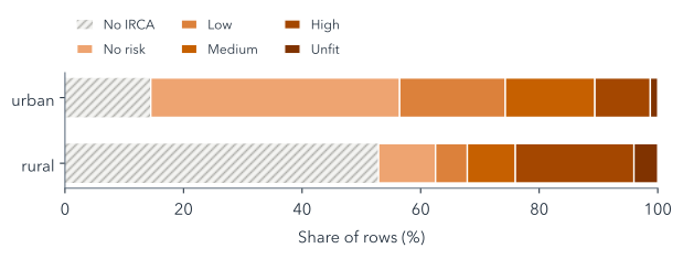
Side by side, Figure 18.1 shows all 31,416 rows. 53% of rural rows have no IRCA at all, against 14% of urban rows, because many rural systems are never sampled, or are not run by a utility and so fall outside the utility-supplied table. Among the rural rows that do have a value, 51% fall in the high or unfit bands, against 12% of urban rows. Those shares pool all fourteen years. In 2023 alone they were 28% and 6%, the figures that open the water analysis, after the falls in rural IRCA that Figure 18.2 shows below.
The two facts compound, in the worst direction: the zones whose scores are worse are also the ones least often scored. The gaps are not random. They depend on zone, which the data record, and perhaps on the risk itself, which they do not: statisticians call the second kind missing not at random, and no fill can repair it. Any analysis that drops the rows without IRCA, as the water analysis’s must, describes sampled rural systems only, and should say so.
Suppose every missing rural IRCA were filled with the median of the scored rural rows. Would rural water then look safer or riskier than it really is?
Probably safer, though nobody can check. Many unscored systems are ones no utility runs, and self-supplied systems score far worse nationally (Table 17.1), so the fill would turn “unknown, and likely worse” into “typical”. That is why the analysis drops these rows instead (Section 19.1).
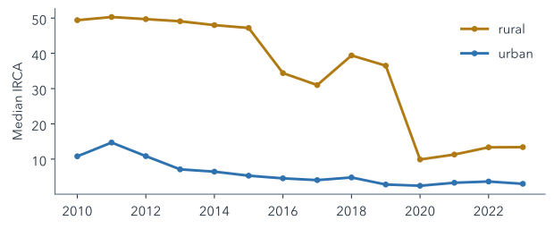
The fourth question matters, as Figure 18.2 shows. The rural median drops sharply in 2016 and again in 2020. That could be an improvement in rural water, or a change in which systems were sampled; the data’s README warns that the 2020 drop may reflect sampling, and the open data cannot tell the two apart. An analysis that compares years should not read the drop as progress without evidence from outside the table.
The rural median also ends far below the national rural figure in Table 17.1: 13.4 in 2023, in the low band, against INCA’s 36.5. Two things explain the gap. The table holds only utility-run systems (Section 17.2), and a median of zones is the middle zone, which the worst zones do not pull up, and which is not weighted by how many people drink the water.
18.3 One municipality to follow: Tunja
Aggregates hide the details that make a variable trustworthy or not, so from here on this part follows one municipality through every step. Tunja, the capital of Boyacá department, is a good case for three reasons in its rows. As a department capital, it carries the coverage caveat that every capital does. Unlike most municipalities, it has an IRCA for both zones in every year: only 117 of the 1,103 municipalities have one for their rural zone in all fourteen years, so the analysis will never lose Tunja for want of a score. And its two zones differ: its rural water scored in the high-risk band every year from 2010 to 2014, while its urban water never scored above 11.9.
Tunja has 28 rows, two zones over fourteen years. Zone variables, such as IRCA, differ between its two rows in a year; municipal ones, such as rainfall and infant mortality, repeat on both (Table 17.2), so the explorer and every summary count them once. Looking at the rows one variable at a time shows several of the README’s caveats in a single place (Figure 18.3).
water_municipal.csv. Pick a view (the data, a summary, a distribution, a time series or a scatter plot), then a variable and a zone. Variables that repeat the same value in both zone rows are municipal and are counted once.
Tunja’s infant mortality drops in 2017. Is that progress?
Not on this evidence. The series changes method that year, from what look like modelled estimates to observed rates (the data’s README, caveat 8), so the drop may be the change itself, and the table cannot tell. A series like this is compared only within one method.
Five things are worth finding (Table 18.1). Because Tunja is a department capital, its coverage has no urban and rural split, so the explorer uses the municipality’s total. That total is reported as exactly 0 in 2021, which beside its neighbouring years probably means “not reported” rather than “no service”; such points are drawn hollow. The fiscal index idf ends in 2020 and idf_new starts there, on a different scale, so the two must never be joined into one line.
data/README.md, as they show in Tunja’s rows, and what the analysis does about each.
| Caveat | In Tunja’s rows | The analysis |
|---|---|---|
| No zone split for capitals’ coverage | the municipal total only | fills it, flagged (Section 19.1) |
| A 0 may mean “not reported” | coverage 0 in 2021 | keeps it (Section 19.2) |
| Two fiscal indices | idf ends in 2020, idf_new starts |
uses neither (Section 17.5) |
| Infant mortality’s new method | a drop in 2017 | 2017–2019 and 2021–2023 only (Section 21.4) |
| Saber 11 in some years | 2014–2017, 2019, 2020 and 2022 | published years only (Section 21.4) |
Summaries in the explorer never pool the two zones. Averaging the small rural population’s values with the much larger urban population’s would describe neither. The same caution applies to every comparison in this part: compare like with like, and say which rows a number comes from.
18.4 The first page: explore.qmd
Read data/README.md. Create explore.qmd from data/water_municipal.csv (divipola as text): rows and columns, % missing per column by `zone`, IRCA counts by Resolución 2115 band and `zone`, and median IRCA by `year` and `zone`, labelled utility-supplied (prestadores). Render it; report errors.writes explore.qmd · uv run quarto render explore.qmd
open explore.html in your browser
“divipola as text” matters: the codes have leading zeros (05001 is Medellín), and a code read as a number loses them, and with them the join to any other table.
Check the missingness table before trusting the page. irca should be missing in about 53% of rural rows and 14% of urban ones. If it is not much sparser in rural rows than in urban ones, the agent probably counted the wrong column, or counted rows rather than values. You now know the answer the table should give (Figure 18.1), which is exactly what makes the check possible.
This catch-up covers Chapter 17 too: it restores the rules and the environment as well as explore.qmd, and copies data/ if it is missing, because the water checkpoints hold sources only.
Summary
- Before modelling, ask a table’s size, what is missing and where, how key values are distributed and how they move over time.
- Rural rows are mostly without IRCA and, where scored, riskier, so results describe sampled systems only.
- The gaps may depend on the risk itself, so filling them would invent water quality nobody measured.
- A jump in a series can be a change of method or sampling, which the table cannot tell from a real change.
- Keep the zones apart, count municipal variables once, and read codes as text.
Seeing the gaps is not the same as deciding what to do about them: the next chapter decides which rows and numbers the clustering will see, and counts what each decision costs.
Further reading
examples/water/data/README.md, “Known gaps and caveats”, in the workshop repository: the full list of the data’s traps, with how each was found.- pandas, Working with missing data (checked 2026-11-12).
- Quarto, Tables: computed and Markdown tables with captions (checked 2026-11-12).