22 Correlation Is Not Causation
Quarto, reproducible publishing, coding agents, Markdown, Python, EPUB, data analysis, k-means clustering
The analysis was built to ask whether places with worse water have worse outcomes, and the temptation, once there is a chart, is to read the answer as an effect: worse water causes more infant deaths. The data cannot support that sentence, and this chapter shows why, with the analysis’s own numbers.
One more comparison, the association between water safety and infant mortality within each kind of place, comes out weak in every kind, and in one as large as across all of them. But neither a strong association nor a weak one could settle the causal question here, and the reasons decide how the results must be written. That last part is not a formality: the sentence a reader quotes is the one you publish.
- Explain what Spearman’s ρ measures, and read it across all places and within each kind.
- Explain why comparing within a cluster holds poverty, rurality and coverage only partly fixed, and why the four values cannot be ranked.
- Name the paths that can create or hide an association here, and say which way each could push.
- Write a result with verbs of association, the rows compared, its limits and what it does not show.
22.1 Worse water, more infant deaths?
The measure is Spearman’s \(\rho\) (rho), which asks whether two variables rise and fall together in rank order: sort the places by each variable, and see whether the two orders agree. It runs from −1 (perfectly opposite) through 0 to +1 (perfectly together), where 0 means no monotonic relation, one in which a variable tends to rise as the other rises, though not necessarily along a straight line. Because it uses ranks, it is not thrown by extreme values, which matters with small municipalities’ noisy rates.
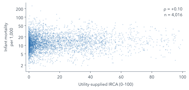
Across all municipality-years with both values in 2017–2019 and 2021–2023, \(\rho\) between utility-supplied IRCA and infant mortality is +0.10 (n = 4,016, the number of municipality-years compared). Figure 22.1 shows what so weak an association looks like: a cloud with no visible slope.
A small positive association across all places could come from water, or from everything that differs between places with safe and unsafe water. The clusters offer a partial control, a way of comparing like with like: within a cluster, places are more alike in poverty, rurality, coverage and altitude than across the country, though far from equal (Table 22.1).
| Feature | 1 | 2 | 3 | 4 |
|---|---|---|---|---|
| Poverty | 0.53 | 0.47 | 0.75 | 0.87 |
| Rural share | 0.79 | 0.58 | 0.89 | 0.85 |
| Piped-water coverage | 0.80 | 0.35 | 0.46 | 0.88 |
| Altitude | 0.93 | 0.69 | 0.40 | 0.96 |
Every value is below 1, but some only just: inside cluster 4, altitude varies almost as much as across all kept zone-years. So the check repeats the comparison inside each cluster (Figure 22.2), where some of the differences between places are smaller.
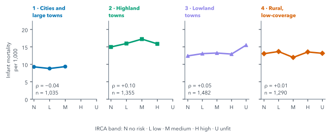
Within the clusters, \(\rho\) runs from −0.04 in cluster 1 to +0.10 in cluster 2, where it is as large as across all places (Table 22.2). These figures cannot be ranked against each other, or set beside the pooled one, at face value, for three reasons.
| n | ρ | 95% interval | SD of IRCA | |
|---|---|---|---|---|
| All places | 4,016 | +0.10 | +0.06 to +0.14 | 20.1 |
| Cluster 1 | 1,035 | −0.04 | −0.11 to +0.05 | 8.5 |
| Cluster 2 | 1,355 | +0.10 | +0.03 to +0.16 | 11.9 |
| Cluster 3 | 1,482 | +0.05 | −0.01 to +0.12 | 22.9 |
| Cluster 4 | 1,290 | +0.01 | −0.06 to +0.07 | 31.1 |
The first is range. The clusters were formed partly on IRCA, so inside clusters 1 and 2 it varies far less than across all places, and inside clusters 3 and 4 more. A narrower range tends to weaken a rank correlation, but that does not explain these four: \(\rho\) is largest in cluster 2, where IRCA varies little, and closest to zero in cluster 4, where it varies most.
The second is chance. To see how far \(\rho\) could move with another draw of places, the book redraws each set’s municipalities 1,000 times, with replacement and keeping each municipality’s years together, and recomputes \(\rho\) every time; the middle 95% of those values is the interval in Table 22.2. Each cluster’s interval reaches 0.06 to 0.08 either side of its \(\rho\), more than the gaps between neighbouring values, so these data cannot rank the four. The intervals for clusters 1, 3 and 4 include zero; the pooled one does not.
The third is the unit, because the unit follows the outcome. Infant mortality is measured for a whole municipality, so each municipality-year counts once, with the mean IRCA of its zones: all of them for the pooled figure, only those in the cluster for a cluster’s. That mean is unweighted, and it covers only the zones with a score: in 54% of the pooled municipality-years only one zone has one. So the IRCA beside a rate is one zone’s score or the plain mean of two, not what the average resident drinks.
It would be easy to read this as “water does not matter”. That reading is as unsupported as the first one.
Within cluster 4, \(\rho\) is close to zero. Write the sentence a councillor might wrongly take from it, and an honest one.
Wrong: “In rural, low-coverage places, water quality makes no difference to infant deaths.” Honest: “Within the rural, low-coverage kind, municipality-years with higher utility-supplied IRCA did not have markedly higher recorded infant mortality (2017–2019 and 2021–2023). This does not show that water has no effect: under-reporting, blank rates and the mismatch between zone and municipality could hide one.”
22.2 What else could explain it
Figure 22.3 draws the paths between water and infant mortality that the data cannot separate.
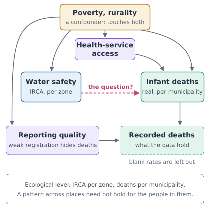
Poverty and rurality are likely confounders. A confounder is a third variable that affects both the exposure, here water safety, and the outcome, here infant deaths, so the two move together even if one has no effect on the other. Poorer, more rural places tend to have less safe water and, for other reasons, more infant deaths, so they can produce an association between water and mortality with no effect of water at all. Health-service access carries part of that path: poorer and remoter places have less of it, and less access means more infant deaths.
Reporting quality is a problem of measurement, and it works the other way: places with weak birth and death registration record fewer infant deaths than occur, and if those are also the places with unsafe water, under-recording can hide a real effect. Blanks add a second problem. The series holds no zeros, so a blank rate may mean no deaths were recorded, and 32% of the clustered municipality-years in these years are blank. Leaving them out drops what may be recorded zeros, which raises small places’ averages most: a selection on the outcome itself (Section 21.4).
Then there is the ecological level. IRCA is measured for an urban or rural zone, infant mortality for the whole municipality. A pattern across places need not hold for the people in them: the infants who died need not be the ones drinking the worst water. Drawing individual conclusions from aggregate data is known as the ecological fallacy.
Tunja shows the mismatch in one place. In this check each of its six municipality-years counts once in cluster 1, with the mean IRCA of its two zones: in 2018, for example, 9.15, halfway between its urban water’s 0.5 and its rural water’s 17.8, a value neither zone had. The mean weighs the two zones equally, though at most 5% of Tunja’s people live in the rural one, and the infant mortality beside it is the whole municipality’s.
The clusters narrow some of these differences without removing them: within a cluster, places still differ in poverty and access (Table 22.1). And small municipalities produce extreme rates, which add noise that flattens any line.
Pick one of these paths. Could it hide a real effect, or create a fake one?
Poverty can create a fake one: if poorer places tend to have both less safe water and, for other reasons, more infant deaths, the two move together without water doing anything. Reporting quality can hide a real one: if unsafe-water places under-record deaths, their measured rates are too low, and a real effect looks smaller than it is. Only the first is a confounder; the second is a problem of measurement. Each path pushes one way, but several act at once and their sizes are unknown, so the net bias could go either way, which is why a correlation cannot settle the question.
Table 22.3 sorts the paths by the kind of problem each one is.
| Problem | Here | Can create a false link? | Can hide a real one? |
|---|---|---|---|
| Confounding | poverty, rurality, health-service access | yes | yes |
| Measurement | weak registration of deaths | yes | yes |
| Selection | blank rates left out | yes | yes |
| Level | IRCA per zone, deaths per municipality | yes | yes |
| Noise | small places’ extreme rates | no | yes |
A causal claim needs a design that handles these paths, not a better chart: for example, comparing places before and after a change in water treatment, against comparable places without the change, a design known as difference-in-differences. That is a different study, with different data; Hernán and Robins, in Further reading, cover such designs.
22.3 Writing it honestly
Every output of this analysis says the same thing in the same words, because the project’s rules require it: comparisons between clusters are descriptive and do not establish a causal effect of water safety. In practice that means a few habits:
- Describe what was compared, and over which rows: “within each cluster, 2017–2019 and 2021–2023, municipality-years with both values”.
- Use verbs of association (“is higher in”, “varies with”), not of effect (“raises”, “reduces”, “leads to”).
- Name the data’s limits beside the result: the utility-supplied IRCA, the method change in infant mortality, the zone-versus-municipality mismatch.
- State what the result does not show, in one sentence a reader could quote.
The causal sentence usually arrives in the last step: a slide title, a blog post’s headline, a summary for a council. Ask the agent to check every title and summary against the project’s rules, and read them yourself. “Utility-supplied water risk (IRCA) and infant mortality in Colombian municipalities” is a fair title; “How unsafe water kills infants” is not, however strongly you suspect it.
22.4 Building the check
The normal route copies the finished check:
Copy ../quarto-workshop/checkpoints/09-water-causation/scripts/analysis.py over scripts/analysis.py (keep mine as scripts/analysis-before-09.py), run it with `uv run python scripts/analysis.py`, and print Spearman rho and n per cluster from outputs/irca_infant.csv.copies · runs · writes outputs/irca_infant.csv and outputs/irca_infant_bins.csv
It should print four rows, one per cluster, with \(\rho\) from −0.04 to +0.10 and n from 1,035 to 1,482, as in Table 22.2.
To build it instead (optional):
In scripts/analysis.py, for 2017–2019 and 2021–2023, make one row per municipality-year within each cluster: its infant_mortality and the mean IRCA of its zones in that cluster. Save and print Spearman rho and n per cluster, and median infant_mortality by IRCA band. Run it.Both routes then show it on the clusters page:
Add a section to clusters.qmd that reads those outputs: median infant_mortality by IRCA band per cluster, with rho and n, and one sentence stating this is descriptive and does not establish a causal effect of water safety. Render it.Summary
- Spearman’s \(\rho\) measures whether two variables rise and fall together in rank order; across all places, utility-supplied IRCA and infant mortality are only weakly associated (\(\rho\) = +0.10).
- Within the clusters, where places are more alike but far from equal, \(\rho\) runs from −0.04 to +0.10; range, chance and a different unit mean these values cannot be ranked or set beside the pooled one at face value.
- Poverty and rurality are likely confounders that can create an association with no effect, while weak reporting and blank rates can hide a real one.
- IRCA is measured per zone and infant mortality per municipality, and reading a pattern across places as one about the people in them is the ecological fallacy, as Tunja’s averaged zones show.
- Neither a strong nor a weak association settles the causal question; that needs a design, such as before-and-after comparisons with comparable places.
- Write about association: name the rows compared, use verbs of association, put the limits beside the result and say what it does not show.
Check every title and summary against that rule before it goes out. Chapter 23 takes the results, and those sentences, to the officials and the council, in every format they need.
Further reading
- C. Spearman, “The proof and measurement of association between two things”, The American Journal of Psychology 15(1) (1904), doi:10.2307/1412159, where the rank correlation was introduced; cited in
examples/water/references.biband checked against its publisher’s page (2026-11-01). - W. S. Robinson, “Ecological correlations and the behavior of individuals”, American Sociological Review 15(3), 351–357 (1950), doi:10.2307/2087176, the classic account of the ecological fallacy; cited in
examples/water/references.biband checked against its publisher’s page (2026-11-01; pages from the paper’s 2009 reprint in the International Journal of Epidemiology, checked 2026-11-12). - Miguel A. Hernán and James M. Robins, Causal Inference: What If (Boca Raton: Chapman & Hall/CRC, 2020; free online), on confounding and designs for causal questions (checked 2026-11-12).
- SciPy,
spearmanr, the rank correlation and its assumptions (checked 2026-11-12).