19 From Table to Features
Quarto, reproducible publishing, coding agents, Markdown, Python, EPUB, data analysis, k-means clustering
A clustering algorithm does not read a table the way a person does. It sees numbers, measures distances between rows, and groups rows that are close. Everything about the result depends on which rows it sees, which numbers, on what scale, and what it is given where a number is missing. Preparation is the name for those decisions, and they shape the clusters as much as the algorithm does. Four of them stand between the water table and the clustering, and each has a price, counted in rows and in guesses.
- Explain the four preparation steps and what each one costs.
- Compute a within-year z-score and say what +1 means.
- Explain why scaling decides what the clusters can see, and why equal weight is a choice.
- Check
prepare()’s counts, and follow one municipality through every step.
19.1 Four steps from table to features
1. Select. Keep the years 2016 to 2023, because the municipal performance index (MDM), one of the features, starts in 2016. Keep municipalities only: San Andrés has none of DNP’s values and the non-municipalised areas are nearly empty. Keep only rows with an IRCA value, since water safety is the point of the analysis. IRCA is the one feature never filled: its gaps may depend on the risk itself (Section 18.2), so a filled score would be a guess at exactly what the analysis is about.
2. Transform. Transfers for water per person (SGP) are heavily skewed: most are moderate and a few are very large. So the analysis uses their logarithm, which measures ratios rather than differences: every doubling of a transfer adds the same amount, and the few very large transfers no longer sit far from all the rest. Department capitals have no urban and rural split for coverage, so their urban rows use the municipality’s total coverage instead, and a flag column records that they did. The total suits the urban row because most of a capital’s people live in its head town (88% in the median capital in 2023). It would not suit the rural row: in other municipalities the total exceeds the rural figure in 86% of rural zone-years, so the capitals’ rural rows are filled in the next step instead.
3. Impute, with flags. To impute is to fill a missing value with an estimate. Drop rows missing more than two of the nine features. Fill the remaining gaps with the median of the same year and zone, and add a flag column, such as water_coverage_imputed, that marks every filled value. The median, because a few extreme values cannot pull it; the same year and zone, because rural and urban zones differ (Section 18.2) and years shift.
4. Standardise within each year. Replace each feature by its z-score within its year:
\[z = \frac{x - \bar{x}_{\text{year}}}{s_{\text{year}}}\]
where \(x\) is a row’s value of the feature, and \(\bar{x}_{\text{year}}\) and \(s_{\text{year}}\) are the feature’s mean and standard deviation over that year’s kept rows. The standard deviation is, roughly, the typical distance of a value from the mean, in the feature’s own unit. A z-score of +1 means one standard deviation above that year’s average; a z-score has no unit.
Why within each year rather than over all years? Two reasons. SGP is in nominal pesos, not adjusted for inflation, so its values drift upwards over time for reasons unrelated to any municipality. And other features shift as a whole from year to year, as rural IRCA does in Figure 18.2. Standardising within each year removes both shifts. A zone is compared only with that year’s other zones, so a nationwide shift, real or an artefact of sampling, does not move it between clusters, and one clustering over all years gives labels that mean the same relative position in every year. The price is that a real improvement shared by every zone is invisible to the clusters too.
Every fill is a guess, and an unflagged guess becomes indistinguishable from data. The flags make the guesses countable and checkable later: a cluster made mostly of imputed values would be a cluster of medians, not of places. The data’s README says it of the capitals’ coverage (“Do not do it silently”), and the project’s AGENTS.md, written from that README, carries its caveats to the agent: nothing is filled silently.
19.2 What the steps keep
Each decision has a price in rows (Table 19.1).
prepare().
| Step | Rows |
|---|---|
| municipality rows, 2016–2023 | 17,648 |
| dropped: no IRCA | 6,411 |
| dropped: more than two features missing | 2 |
| kept: 7,534 urban and 3,701 rural | 11,235 |
The kept rows cover 1,090 municipalities. 653 rows have at least one imputed value, and 214 urban rows of department capitals took the municipal total for coverage.
Almost all the loss is the first drop: rows without an IRCA value, most of them rural zones that are never sampled or have no utility (Section 18.2). So the rural cluster that appears in the next chapter describes sampled rural systems only. The imputed values are coverage values: the rural rows of capitals, and municipalities whose split is missing in some years.
Tunja shows both treatments of a capital, and loses none of its 16 zone-years from 2016 to 2023. Its 8 urban rows took the municipal total for coverage, flagged in water_coverage_from_total, and its 8 rural rows took the rural median of their year, flagged in water_coverage_imputed. The check also turns up something the flags do not mark: the total that the urban row for 2021 took is the 0 that the Tunja section (Section 18.3) flagged as probably “not reported”. The analysis keeps it as published, as the data’s README does. Treating such zeros as missing would be a defensible change, but one to make in prepare() and report, never silently.
Suppose prepare() treated Tunja’s reported 0 as missing. What would happen to that row, and to its coverage z-score?
With no total to take, the urban row for 2021 would go to step 3 and be filled with that year’s urban median, flagged in water_coverage_imputed. Its coverage z-score would move from −1.9, far below the year’s average, to about +0.8, an ordinary head town’s: an unflagged error would become a flagged guess.
19.3 Why scale?
k-means groups rows by straight-line, or Euclidean, distance: the square root of the sum of squared differences across the features. A feature’s share of the expected squared distance, between two rows picked at random, is proportional to its variance, the square of its standard deviation. In raw units, the features measured in thousands, such as millimetres of rain and metres of altitude, dwarf those measured from 0 to 100 (Figure 19.1).
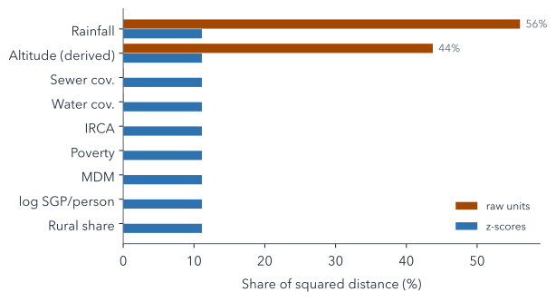
Unscaled, rainfall and altitude together would make up 99.8% of the distance, so the clusters would be climate zones and the water variables would hardly count. After z-scores, every feature has variance 1 and contributes the same share, about 11%. The log of SGP matters too. In raw pesos, its variance would be about 3,100 times rainfall’s, so it would dominate even rainfall; after z-scores, the log keeps a few very large transfers from sitting far from every other row, cutting the largest z-score from 7.3 to 4.3.
Two real rows show what scaling changes (Table 19.2): the urban zones of Tunja, high in the Andes, and Cartagena, on the Caribbean coast, in 2023. Both are capitals, so their coverage is each municipality’s total. In raw units, their difference in altitude makes up 98% of their squared distance, and a 43-point gap in piped-water coverage makes up less than 1%. In z-scores, coverage counts for 16%, and altitude still leads, at 68%, because height is where the two towns really differ most. Scaling does not make every difference count the same; it stops the units from deciding.
| Feature | Difference | Share, raw | Share, z |
|---|---|---|---|
| IRCA | 0.0 | 0% | 0% |
| Water cov. | 43.4 | <1% | 16% |
| Sewer cov. | 41.7 | <1% | 8% |
| Poverty | 7.9 | <1% | 2% |
| Rural share | 0.06 | <1% | 1% |
| Altitude (derived) | 2,679 m | 98% | 68% |
| Rainfall | 416 mm | 2% | 2% |
| MDM | 0.5 | <1% | <1% |
| log SGP/person | 0.39 | <1% | 3% |
Suppose rainfall were recorded in metres instead of millimetres. What would happen to its share of the distance, unscaled and after z-scores?
Unscaled, its values would shrink a thousandfold and its variance a millionfold, so its share would all but vanish and altitude would dominate alone. After z-scores nothing would change: the unit cancels, because a z-score divides a distance from the mean by the standard deviation, both in the same unit.
Equal weight is itself a choice, not a neutral default. Nine z-scored features count equally, so the three safety-and-coverage variables count for 33% of the distance and context for the rest. Equal weight per feature is not equal weight per idea, either: water and sewer coverage are strongly correlated (r = 0.77 over the kept rows, where the correlation coefficient r runs from −1 to 1 and 1 would mean they rise together along a straight line), so what they share counts twice. If water safety should weigh more, that is a decision to make explicitly and report, not to leave to the units the data happened to come in.
19.4 Building prepare()
Two prompts write the four steps into the project’s script. The first selects and transforms:
Read data/README.md. Create scripts/analysis.py with prepare(df): rows with entity_type "municipality", 2016–2023, with irca; features irca, water_coverage, sewer_coverage, ipm, rural_share, altitude_m, rainfall_mm, mdm, log(sgp_water_pc); fill missing coverage of "urban" rows with department_capital == 1 from *_total, flagged in <col>_from_total. Run it.writes scripts/analysis.py · uv run python scripts/analysis.py
You should see it run without errors and, if it reports a count, 11,237 rows: the municipality rows for 2016–2023 that have an IRCA value, before any are dropped for missing features. department_capital, which this prompt relies on, marks the 32 department capitals. The build script writes it from the DIVIPOLA codes, where each capital is numbered 001, except that Cundinamarca’s capital is Bogotá, so 25001 (Agua de Dios) is not one: a detail the agent can only get right by reading the data’s README.
The second imputes and standardises, and saves the result:
In prepare(), drop rows missing more than 2 features, fill the rest with the `year` × `zone` median plus <col>_imputed flags, then add z_<col> (z-score within `year`) beside the original columns; keep keys, outcomes and flags. Save outputs/prepared.parquet, print rows kept and dropped per step. Run it.edits prepare() · uv run python scripts/analysis.py
The finished project’s version of the imputation and scaling, slightly trimmed, shows how little code each decision takes once it is clear:
n_missing = d[FEATURES].isna().sum(axis=1)
1d = d[n_missing <= MAX_MISSING].copy()

2medians = (d.groupby(["year", "zone"])[FEATURES]
           .transform("median"))
for col in FEATURES:
3    d[f"{col}_imputed"] = d[col].isna().astype(int)
    d[col] = d[col].fillna(medians[col])

4grp = d.groupby("year")[FEATURES]
z = ((d[FEATURES] - grp.transform("mean"))
/ grp.transform(lambda s: s.std(ddof=0)))- 1
-
MAX_MISSINGis 2, set once at the top of the script; the water analysis’s last exercise changes it. - 2
- The median of each feature within the same year and zone, aligned with every row.
- 3
- The flag is written before the fill, so it records exactly which values were missing.
- 4
- Means and standard deviations by year: the within-year z-scores of the formula above.
Summary
- Which rows, which numbers, how gaps are filled and on what scale shape the clusters as much as the algorithm.
- The largest price is the rows without IRCA, so rural results describe sampled systems only.
- Every fill carries a flag, yet a check can still find a value no flag marks.
- Within-year z-scores put the features on one scale and remove nationwide shifts.
- Unscaled, rainfall and altitude would decide the clusters; equal weight is itself a choice.
What is left is 11,235 rows of nine z-scores each, too many for anyone to read: the next chapter asks an algorithm to summarise them in a few kinds.
Further reading
- scikit-learn, Preprocessing data: standardisation (checked 2026-11-12).
- scikit-learn, Imputation of missing values, including indicator columns that mark imputed values (checked 2026-11-12).
examples/water/scripts/analysis.py,prepare(), in the workshop repository: the full function, with its counts.