20 Finding Kinds of Places: k-Means
Quarto, reproducible publishing, coding agents, Markdown, Python, EPUB, data analysis, k-means clustering
The water data now have 11,235 prepared rows, each described by nine z-scores. Nobody can read that many rows. Clustering turns them into a few kinds that a person can name, compare and act on: these municipal zones are like each other, and unlike those. An official can ask which kinds need which help; a council can see which kind its own zones belong to. Clustering needs no labels, so it is a first look at data nobody has categorised, and an odd cluster can point to a data error or a special case. What it cannot do is explain: clusters describe, they do not show causes.
If the mathematics sounds daunting, it need not be. The algorithm is simple enough to watch step by step, and the judgement it needs, how many kinds to look for, is a decision you can write down and check before seeing the answer.
- Describe the k-means loop, and why it needs many starts and a fixed seed.
- Apply the written rule for k, and say how close the call was.
- Interpret a low silhouette, a stability check and a PCA picture without over-reading them.
- Run the clustering step and check the agent’s account of k.
20.1 k-means in four steps
k-means needs one number up front: \(k\), how many clusters to find. It makes one start, then repeats two moves until they change nothing:
- Drop \(k\) centres at \(k\) randomly chosen data points.
- Assign every point to its nearest centre.
- Move each centre to the mean of the points assigned to it.
- Repeat 2 and 3 until nothing changes.
Neither move ever raises the inertia, the sum of squared distances from each point to its centre,
\[\text{inertia} = \sum_{i} \lVert x_i - c_{\ell(i)} \rVert^2 ,\]
where \(x_i\) is point \(i\) (for the water data, a row’s nine z-scores), \(c_{\ell(i)}\) is the centre it is assigned to, and \(\lVert x_i - c_{\ell(i)} \rVert\) is the straight-line distance between them (Section 19.3). On z-scores, inertia is in squared standard deviations, a unit with no everyday meaning, so only its changes matter. There are only finitely many ways to group the points, so the algorithm always stops. It does not always stop at the best answer: a bad start can trap it in a worse grouping. Figure 20.1 shows the algorithm on 560 synthetic points in three groups, which are toy data made up for the illustration, not the water data.
This 3-D view needs WebGL. The four steps are listed above.
1. drop 3 centres at random points
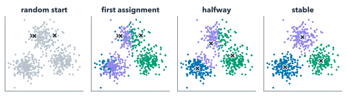
Different starts can end in different groupings, so the real analysis runs k-means from 20 starts (scikit-learn’s n_init) and keeps the one with the lowest inertia. The starts are random, but repeatable: a fixed random seed, the number that starts the computer’s random-number generator, makes them the same on every run, so your project, the deck and this book all get the same clusters.
The real starts are not dropped at random, as in the toy. scikit-learn’s default, k-means++ (Arthur and Vassilvitskii, 2007), picks the first centre at random from the data and each next one with probability proportional to its squared distance from the nearest centre already chosen. That spreads the centres out and makes a stuck start less likely; scikit-learn uses a greedy variant that draws several candidates at each step and keeps the best.
20.2 Choosing k
k is a hyperparameter: a setting the algorithm cannot learn from its own objective, because inertia always falls as k grows, down to zero when every point is its own cluster. So the analysis fits k-means for k from 2 to 8 and reads two measures (Figure 20.3). The first is where inertia stops falling much, the elbow. The second, the silhouette, scores from −1 to 1 how much closer each point is to its own cluster than to the next one, averaged over the points. It needs every distance between points, so it is computed on a fixed sample of 5,000 rows, which keeps it fast.
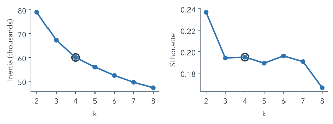
The rule, written into choose_k() in the analysis script, has three parts, and Table 20.1 applies it row by row:
- k = 2 is excluded. Two clusters mostly split urban from rural rows, which we knew already: they match the zone for 86% of rows. The script measures this with the adjusted Rand index (ARI), which scores how far two groupings agree beyond what chance would give: 1 means identical, 0 no better than chance. Here it is 0.50.
- The elbow: take the smallest k from 3 up after which one more cluster cuts inertia by less than 10%. Here that is k = 4: a fifth cluster cuts inertia by only 7%.
- The silhouette check: k’s silhouette must be within 0.01 of the best for k ≥ 3. At k = 4 it is 0.195. The check rules out only k = 8 here.
choose_k()’s rule, row by row, on the kept rows: how much one more cluster would cut inertia, the silhouette (on the fixed sample) and the verdict. Computed by the finished project’s analysis.py.
| k | One more cluster cuts | Silhouette | Verdict |
|---|---|---|---|
| 2 | 14.9% | 0.237 | excluded: the urban–rural split |
| 3 | 10.8% | 0.194 | one more still cuts 10% or more |
| 4 | 6.7% | 0.195 | chosen: the smallest that passes |
| 5 | 6.3% | 0.189 | passes, but larger |
| 6 | 5.4% | 0.196 | passes, but larger |
| 7 | 4.7% | 0.191 | passes, but larger |
| 8 | – | 0.166 | silhouette too far below the best |
The elbow is marginal. The fourth cluster itself cuts inertia by 10.8% (the row for k = 3), only just above the 10% threshold, so a threshold of 11% would pick k = 3 instead. And the four clusters account for 41% of the spread in the data, one minus the ratio of their inertia to that of a single cluster; the rest is difference within the kinds.
Two more checks follow the fit. Stability: refits from 5 other seeds agree, with an adjusted Rand index of at least 0.998, so the result does not depend on the start. That says nothing about other data, features or k; refitting on rows drawn again at random (a bootstrap), or leaving out one year at a time, would test that. Ordering: clusters are numbered by their centre’s IRCA, from lowest to highest, so a re-run keeps the same numbers and colours.
A silhouette near 0.2 is low. In the subjective reading Rousseeuw and colleagues propose, a best average silhouette of 0.25 or less means that “no substantial structure has been found” (Struyf, Hubert and Rousseeuw, 1997, Table 2), and the best here, at any k, is 0.24. The kinds overlap: they summarise a continuum rather than separate islands of data. So treat k as a judgement call, and do not force a number of clusters to make a nicer story. Writing the rule down before seeing the result is what keeps such a choice honest; choose_k() at least makes the rule explicit, so anyone can check it and see how close the call was.
An official reads the report and asks: “So Colombia has four kinds of municipal zone?” What do you answer?
That four is a useful summary, not a discovery. A written rule chose it by a narrow margin, and a threshold one percentage point higher picks three; the low silhouette says the kinds overlap. The clusters describe typical combinations of water, services and context, and a zone near the edge of one could as well sit in the next.
20.3 A picture of the clusters
Nine dimensions cannot be drawn. Principal component analysis (PCA) finds the directions in which the data vary most and projects the rows onto them. Each direction, a principal component, is a weighted sum of the nine z-scores, and its weights, called loadings, say what it measures. Figure 20.4 uses the first two components, which keep 30% and 21% of the variance.
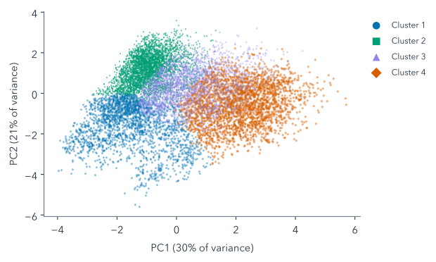
Overlaps in the picture can be separations in the dimensions it leaves out. Adding a third component, which keeps another 16% of the variance, shows how much (Figure 20.5). On two components, on average 78% of a zone-year’s 15 nearest neighbours are in its own cluster; on three, 94%. The third component rises with altitude and falls with rainfall, its two largest loadings. Cluster 3, the most mixed in two dimensions, sits below the others along it: it is the lowest and wettest of the kinds.
This 3-D view needs WebGL. The 2-D picture is the figure above.
20.4 Where the clusters stand
Altitude carries the third component’s largest loading. A map shows altitude directly (Figure 20.6): one column for each of the 966 clustered urban zones in 2023, at its municipality’s centroid, as tall as its head town’s altitude (one derived SRTM point, exaggerated 50 times) and coloured by cluster.
This 3-D view needs WebGL. Median head-town altitude, 2023 urban zones: cluster 1: 1,256 m; cluster 2: 1,766 m; cluster 3: 130 m; cluster 4: 159 m.
Cluster 2’s urban zones stand highest, with a median altitude of 1,766 m, and 56% of them are in the region Centro Oriente (DANE’s regional grouping). Cluster 3’s stand lowest, at 130 m, and 53% of them are in Caribe. This shows where the kinds are, not why they differ. Tunja’s head town stands at 2,695 m, and all 16 of its zone-years, urban and rural, fall in cluster 1.
The map draws urban zones only, one column per municipality, because the altitude is the head town’s. So it shows little of cluster 4, whose zone-years are 91% rural. Its few urban columns stand low, at a median of 159 m, but the median head-town altitude of its rural zone-years is 1,475 m, so the map says little about where that kind is found.
20.5 Use the model, or build it
There are two routes through the modelling, and both end with the same outputs/ and the same pages:
- Use it (the normal route): copy the finished
analysis.pyfrom this step’s checkpoint, run it, and spend your effort on checking what it chose and on the publications. - Build it (a challenge): give the agent the prompt below and have it write the clustering step itself.
This is a book about publishing, so using the finished model is the normal route, not a fallback. But a copied script is only as trustworthy as your reading of it, so the route has two prompts: one runs the script, the other makes the agent explain what it printed.
Copy ../quarto-workshop/checkpoints/07-water-cluster/scripts/analysis.py over scripts/analysis.py (keep mine as scripts/analysis-before-07.py), run it with `uv run python scripts/analysis.py`, and tell me k.copies the script, keeping yours · uv run python scripts/analysis.py · reports k = 4
Among its output, the script prints the table behind Figure 20.3 and then its verdict in one line, which on this book’s data reads:
k = 4: the next cluster cuts inertia by only 7% (< 10%), and its silhouette 0.195 is within 0.01 of the best k >= 3 (0.196).
Ask the agent to take that line apart:
Explain what scripts/analysis.py printed about k: what `inertia`, `silhouette`, ari_vs_zone and inertia_drop mean for each k, and which test in choose_k() chose k. Quote the lines of choose_k() that decide it.reads the printed table and choose_k() · explains each column and the rule, quoting the code
While it explains: which test in choose_k() chose k, and which could only have ruled one out?
The elbow chose it: k = 4 is the smallest k from 3 up after which one more cluster cuts inertia by less than 10%. k = 2 is excluded before any test, and the silhouette check only vetoes: it rules out only k = 8 here. Check the agent’s explanation against this and Table 20.1: one that says the silhouette chose k has misread the rule.
To build it instead (optional):
In scripts/analysis.py, run k-means on the z_ features for k=2–8 (random_state=42, n_init=20); save inertia and silhouette to outputs/k_selection.csv; pick k by the elbow, check silhouette and 5-seed ARI; number clusters by centroid IRCA; save outputs/clusters.parquet (prepared columns + `cluster`, pc1, pc2). Run it; explain k.If you build it, your k may differ from 4 when your preparation differs, and that is fine if the reason is sound. What matters is that the rule for choosing k is written down before you see the answer, and that the clusters are numbered by a fixed rule (here, centre IRCA, which the prompt calls centroid IRCA), so a re-run keeps the same numbers and colours.
20.6 The clusters page
Both routes then build the project’s second page, which only reads outputs/ and never refits:
Create clusters.qmd that reads outputs/k_selection.csv and outputs/clusters.parquet and shows an elbow plot, silhouette by k and a PCA scatter (pc1, pc2) coloured by cluster, each with a caption and alt text. Render it and tell me about errors.writes clusters.qmd · uv run quarto render clusters.qmd
open clusters.html in your browser
Summary
- k-means assigns points to the nearest centre and moves centres to their points’ mean; it can stall, so it keeps the best of many seeded starts.
- k is chosen by a rule written beforehand: exclude k = 2, take the elbow, let the silhouette veto.
- The elbow is marginal and the silhouette low: the kinds summarise a continuum.
- Agreement across seeds shows independence from the start, not from the data or features.
- PCA and the map show where the kinds stand, not why, and the map leaves rural zone-years out.
- Using the finished model is legitimate if you can explain what it chose.
The kinds so far are only numbers, from cluster 1, lowest centre IRCA, to cluster 4: the next chapter works out what sets each one apart, names it by a rule, and compares the outcomes the clustering never saw.
Further reading
- scikit-learn, Clustering: k-means and silhouette analysis (checked 2026-11-12).
- scikit-learn, Principal component analysis (checked 2026-11-12).
- Stuart P. Lloyd, “Least squares quantization in PCM”, IEEE Transactions on Information Theory 28(2), 129–137, 1982, https://doi.org/10.1109/TIT.1982.1056489: the algorithm behind k-means (checked 2026-11-12).
- Peter J. Rousseeuw, “Silhouettes: a graphical aid to the interpretation and validation of cluster analysis”, Journal of Computational and Applied Mathematics 20, 53–65, 1987, https://doi.org/10.1016/0377-0427(87)90125-7: the silhouette (checked 2026-11-12).
- Anja Struyf, Mia Hubert and Peter Rousseeuw, “Clustering in an object-oriented environment”, Journal of Statistical Software 1(4), 1997, https://doi.org/10.18637/jss.v001.i04: Table 2 reads the silhouette coefficient (checked 2026-11-12).
- David Arthur and Sergei Vassilvitskii, “k-means++: the advantages of careful seeding”, SODA 2007 (ACM-SIAM Symposium on Discrete Algorithms), https://theory.stanford.edu/~sergei/papers/kMeansPP-soda.pdf (checked 2026-11-12).
examples/water/references.bibin the workshop repository: the k-means, silhouette and adjusted Rand index papers the finished white paper cites, checked against their publishers’ pages.