17 The Question, the Data and the Rules
Quarto, reproducible publishing, coding agents, Markdown, Python, EPUB, data analysis, k-means clustering
In 2023, Colombia’s national report on drinking water scored the water of its urban areas at 5.7, in the low-risk band, and the water of its rural areas at 36.5, in the high-risk band (Table 17.1). DANE’s projections put 12.6 million people, 24% of the population, in rural zones in 2023. People drink and cook with this water, so where the risk sits, and what goes with it, is worth knowing.
The question for this part is therefore: which kinds of municipal zone exist in Colombia, judged by water safety, services and context, and how do health and education outcomes differ between them? Part II’s numbers were simple counts; these are not. Every step has a way to go wrong that a clean render will not reveal: a variable that means something narrower than its name, a gap that is not random, a comparison that looks causal and is not.
- Explain what the IRCA scores, and why this part’s IRCA understates risk.
- Identify the unit of analysis, and say what an empty cell means.
- Distinguish features from outcomes, and explain why clustering on an outcome is circular.
- Set up the water project’s data, rules and environment.
17.1 The question and its readers
The question splits in two, and the order matters:
- Which kinds of municipal zone exist, judged by water safety, services and context?
- How do health and education outcomes differ between those kinds?
“Kinds” will be clusters: groups of zone-years, each one municipality’s urban or rural zone in one year (Section 17.4), that are similar to each other on the chosen variables, found by an algorithm called k-means (Chapter 20). Because the unit is a zone in a year, a municipality’s two zones can belong to different kinds, and a zone can move between kinds over the years.
The answer has two readers. Officials will read it as a report, in Word or as a PDF, and a municipal council will see it as a short deck of slides (Chapter 23). Both will look for where to act, and both will be tempted to read a difference between kinds as an effect of the water. So the limits are stated now, each with its reason. The water score covers only systems run by a utility (Section 17.2). Many rural zones have no score at all, so the results describe sampled systems (Section 18.2). And the comparisons describe; they cannot establish that water causes any outcome (Chapter 22).
17.2 Scoring water risk: the IRCA
Colombia scores the safety of drinking water with the IRCA, the Índice de Riesgo de la Calidad del Agua para consumo humano (water-quality risk index for human consumption), defined in Resolución 2115 of 2007. It runs from 0, every test passed, to 100, every test failed, and article 15 sorts the scale into five bands (Table 17.1).
| IRCA | Band | National figures for 2023 that fall in it |
|---|---|---|
| 0–5 | no risk (sin riesgo) | |
| 5.1–14 | low (bajo) | urban areas 5.7; utility-supplied 7.4 |
| 14.1–35 | medium (medio) | the whole country 16.4 |
| 35.1–80 | high (alto) | rural areas 36.5; self-supplied 43.7 |
| 80.1–100 | unfit (inviable sanitariamente) |
The national average sits in the medium band and hides the urban–rural gap, which is why this part’s data keep each municipality’s two zones apart.
Surveillance samples of tap water are tested against health limits. Each tested characteristic carries a risk score: Escherichia coli 25, total coliforms 15, turbidity 15, free residual chlorine 15, apparent colour 6 and pH 1.5, among others. A sample’s IRCA is the score of the characteristics that fail their limit, as a percentage of the score of all those tested, and a month’s IRCA is the mean over its samples (articles 13 and 14). That is why 0 means every test passed and 100 means every test failed.
The IRCA in this part’s data is not the national figure. The open table it comes from (INS, datos.gov.co nxt2-39c3) holds the utility-supplied (“prestadores”) IRCA: samples from systems run by a water utility. A check on 2026-10-30, recorded in the data’s README (caveat 1), found that its 2023 department totals match INCA’s utility column in 30 of 30 departments and the overall figure in only 5. Self-supplied systems, which have no utility, score far worse (43.7 against 7.4 in 2023), so the data understate the risk wherever people rely on self-supply, and say nothing where no utility exists. Label the variable “utility-supplied IRCA” everywhere it appears.
17.3 Saber 11, and what an average covers
One of the outcomes the analysis compares (Section 17.5) is an education measure, Saber 11, the national exam taken by students finishing upper secondary school, set by ICFES. It has five tests: critical reading, mathematics, social studies and citizenship, natural sciences, and English. The global score is five times the weighted mean of the five test scores (each 0 to 100; English counts once, the others three times), from 0 to 500, and its mean was fixed at 250 in the first sitting in 2014, so that years can be compared (ICFES, Guía de orientación Saber 11.° 2017-1, pp. 101 and 104, checked 2026-10-30).
Both measures are averages, and an average describes only what it averaged over. IRCA is an average over the water samples taken, so a system that is never sampled has no IRCA at all. The Saber 11 mean in the data is an average over the students who sat the exam at schools in that municipality and zone, so it says nothing about students who had left school. Keep both facts in mind in every comparison that follows.
17.4 Where the data come from
Most of the data are Colombian open data from five public bodies; rainfall and altitude come from two scientific datasets. All are joined on one code: joining two tables matches their rows by a column they share, here the code that DANE’s list of municipalities, DIVIPOLA (División Político-Administrativa), gives each municipality. It has five digits, two for the department and three for the municipality, so 05001 is Medellín, in Antioquia (05). The sources are:
- INS (Instituto Nacional de Salud): the IRCA surveillance results.
- DANE (the national statistics office): the list of municipalities and their codes, population projections and municipal boundaries.
- ICFES and MEN (the Ministry of Education): Saber 11 results and school dropout rates.
- DNP (the National Planning Department), through its TerriData portal: water and sewer coverage, multidimensional poverty, municipal performance, transfers for water and infant mortality.
- CHIRPS (the Climate Hazards Center’s rainfall data) and NASA SRTM (elevation data): rainfall, and a derived altitude for each head town.
They arrive as three files, in examples/water/data/ in the workshop repository: water_municipal.csv (the analysis table), municipios.geojson (municipal boundaries for maps) and README.md, which documents every column, source, licence and caveat (Appendix G lists them all).
One row is one municipality’s urban or rural zone in one year, a zone-year: this is the analysis’s unit. The urban zone is the head town (cabecera municipal); the rural zone is the smaller settlements and the dispersed countryside. The table covers every one of DANE’s 1,122 DIVIPOLA entries, both zones and every year from 2010 to 2023: 31,416 rows and 29 columns. Of those entries, 1,103 are municipalities; the rest are the island of San Andrés and areas that are not municipalities, whose rows are mostly empty. Because every municipality has all its rows, a gap is an empty cell, never a missing row.
A municipality’s rural zone has no IRCA in one year. Was its water safe that year?
The data cannot say. IRCA averages the samples taken from utility-run systems, so an empty cell means no utility-supplied score was published: the zone may not have been sampled, or its water may be self-supplied, which nationally scores far worse (Table 17.1). An empty IRCA is unknown, never safe and never zero.
Read data/README.md before you analyse anything, and ask the agent to read it first too. Its caveats are the analysis’s traps, written down: the IRCA source above; department capitals that have no urban and rural split for coverage; a fiscal index whose method changes in 2020; infant mortality whose method changes in 2017; Saber 11 only in some years; pesos that are not adjusted for inflation. Each one turns up in the chapters that follow.
17.5 Features and outcomes
The most important design decision in the water analysis is which variables define the kinds and which only describe them.
The features, which the clustering sees, are nine variables about water, people and place, and government. The outcomes, which the analysis only compares, are infant mortality, the Saber 11 score and school dropout (Table 17.2, Table 17.3). Three features need a word. The multidimensional poverty index (IPM, Índice de Pobreza Multidimensional) is the share of a zone’s people who are poor in several respects at once, from the 2018 census. MDM (Medición de Desempeño Municipal) is DNP’s score of a municipality’s management and results. And SGP (Sistema General de Participaciones) is the system of national transfers to municipalities: the feature is its allocation for drinking water and basic sanitation, per person.
Both tables give each variable’s level and years, computed from the municipalities’ rows. A zone variable differs between a municipality’s urban and rural rows; a municipal one is the same on both; “one value” is repeated every year. Meanings, units and sources come from data/README.md (TerriData is DNP’s data portal).
| Variable | Measures (unit); source | Level; years |
|---|---|---|
IRCA (irca) |
water-risk index, utility-supplied (0–100); INS | zone; 2010–2023 |
Piped water (water_coverage) |
aqueduct coverage (%); TerriData | zone; 2010–2023 |
Sewer (sewer_coverage) |
sewerage coverage (%); TerriData | zone; 2010–2023 |
Poverty (ipm) |
people multidimensionally poor (%); 2018 census | zone; one value |
Rural share (rural_share) |
rural share of the population (0–1); DANE | municipality; 2010–2023 |
Altitude (altitude_m) |
the head town’s height (m); SRTM | municipality; one value |
Rainfall (rainfall_mm) |
rain over the municipality (mm a year); CHIRPS | municipality; 2010–2023 |
MDM (mdm) |
municipal performance score (0–100); TerriData | municipality; 2016–2023 |
SGP (sgp_water_pc) |
water transfers (nominal pesos per person, logged); TerriData, DANE | municipality; 2010–2023 |
| Variable | Measures (unit); source | Level; years |
|---|---|---|
Infant mortality (infant_mortality) |
deaths under one year per 1,000 live births; TerriData | municipality; 2010–2023 |
Saber 11 (saber11_mean) |
mean exam score of the zone’s schools (0–500); ICFES | zone; 2014–2017, 2019, 2020 and 2022 |
School dropout (dropout_rate) |
public-school pupils who leave during the year (%); MEN | municipality; 2011–2023 |
The last column matters in every chapter that follows. A zone variable is measured separately for a municipality’s urban and rural zones; a municipal one is a single value for the whole municipality, repeated on both of its rows. Five of the nine features are municipal, so a municipality’s two rows in a year differ only in the other four. And a municipal outcome, such as infant mortality, must be counted once per municipality, not once per row.
Never cluster on an outcome. If infant mortality helped define the kinds, the kinds would differ in infant mortality by construction, and the comparison in the second question would be circular: it would find exactly what was put in. Keeping outcomes out of the clustering is what lets the comparison say anything at all.
A colleague wants infant mortality added to the features, “since it is what we care about”. What would the comparison of outcomes between the kinds then show?
That the kinds differ in infant mortality, which would be true by construction: the algorithm would have grouped zones partly by that very number. The comparison would find what was put in. Infant mortality stays an outcome, compared only after the kinds are found.
The same care is why the fiscal index idf is not a feature, although it describes municipal government: its method changes in 2020 (idf to 2020, idf_new from 2020, on different scales), so it cannot form one series across the years the analysis uses. A variable that changes meaning partway through would create kinds that are artefacts of the change.
17.6 Compute once, publish many
Part II computed in each page. The water analysis computes once (Figure 17.1). One importable script, scripts/analysis.py, does all of the computation and writes its results to outputs/; every page only reads those results and draws them. A design choice, such as how many rows to drop for missing values, is made in one place, and every output follows at the next render.
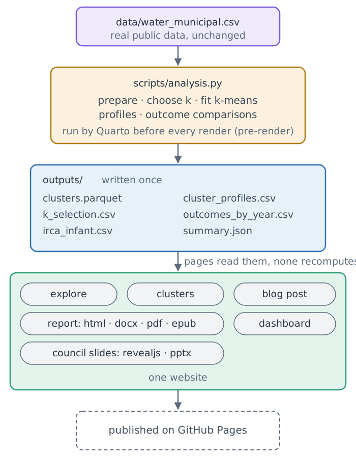
The split solves two problems from Part II. A slow computation no longer slows every page and every format, because it runs once. And no page can disagree with another, because there is only one result to disagree with. Results are saved as Parquet, which keeps column types (a code such as 05001 stays text instead of becoming the number 5001), and as CSV where people will open them.
This book follows the same rule: every number in the water analysis is computed when the book is built, by importing the finished project’s analysis.py and running it in memory.
17.7 Setting up the project: data, rules and environment
The project lives beside the London one, so that the workshop repository’s checkpoints are always at ../quarto-workshop/checkpoints/:
~
├── quarto-workshop/
├── london-guide/
└── water-quality/
In your home folder (~), quarto-workshop/ is the clone from Chapter 4, london-guide/ is Part II’s project and water-quality/ is this part’s.
Quit the London guide’s agent first (/exit), so that the new one starts in the new folder and takes it as its world (Section 2.4). Then make the folder, start its history as you did for the guide (Section 6.2), start the agent in it, and copy the data:
cd ~
mkdir -p water-quality
cd water-quality
git init -b main
claudeCopy ../quarto-workshop/examples/water/data into this folder as data/, then list the files in data/ with their sizes.copies the folder · lists README.md, municipios.geojson and water_municipal.csv with their sizes
The data sit outside the new folder, in ../quarto-workshop/, so the agent asks before it reads there: approve it, as for the London guide (Section 6.2).
Then write the rules. If you have never clustered anything, the worry is fair: the agent can write an analysis that runs, renders and is wrong. You do not guard against that by writing the code yourself. You guard against it by checking, and a check needs something to check against.
Read data/README.md, then create AGENTS.md for this project. Scope: describe Colombian municipal water safety and infant mortality from data/ only. Rules: keep data/ unchanged, label IRCA as utility-supplied (prestadores), never cluster on outcomes, and say comparisons are descriptive, not causal. Show me the file.reads data/README.md · writes AGENTS.md: scope, rules, the data’s caveats
approve · check that AGENTS.md holds all four rules
The four rules are this chapter in miniature: the inputs are evidence and stay unchanged; the IRCA is labelled for what it is; outcomes describe the clusters but never define them; and comparisons between clusters do not establish causal effects of water safety. Asking the agent to read the README first lets it add the data’s caveats to the rules itself.
Give this project its own Python environment with `uv`: run `uv init --bare`, then `uv add ipykernel nbclient nbformat pyyaml pandas numpy matplotlib plotly scikit-learn pyarrow itables tabulate`. Run `quarto` and `python` through `uv run`, and add that rule to AGENTS.md. Create a .gitignore for .venv/, .quarto/, _site/, outputs/ and *_files/. Show me the Python line of `uv run quarto check jupyter`.uv init --bare · uv add … · writes pyproject.toml, uv.lock and .venv/ · adds the uv run rule to AGENTS.md · writes .gitignore · uv run quarto check jupyter
You should see a Python whose path runs through this folder’s .venv, as for the London guide (Section 6.10). The recipe is the London guide’s, with the analysis’s packages added: scikit-learn for k-means, pyarrow for Parquet, itables for the dashboard’s searchable table and tabulate for tables written as Markdown. Packages shared with Part II come from uv’s cache.
Summary
- First find kinds of municipal zone from water, services and context; then compare outcomes between them.
- The data’s IRCA is utility-supplied, so it understates risk wherever people rely on self-supply.
- One row is a zone-year and every row exists, so an empty cell means unmeasured, never safe.
- Zone variables differ between a municipality’s two rows; municipal ones are counted once.
- Features define the kinds and outcomes only describe them: clustering on an outcome is circular.
- One script computes every result once, and
AGENTS.mdholds the limits for the agent.
What the rules cannot say is what the table holds: where it is empty, and where a series moves for reasons unrelated to water. That is the next chapter’s question.
Further reading
- Ministerio de la Protección Social and MAVDT, Resolución 2115 de 2007 (checked 2026-10-30).
- MinSalud, MinVivienda, INS and Superservicios, Informe Nacional de Calidad del Agua para Consumo Humano INCA 2023 (checked 2026-10-30).
- ICFES, Guía de orientación Saber 11.° 2017-1 (checked 2026-10-30).
- datos.gov.co and DNP TerriData, the sources’ portals; every table, licence and cut-off date is in
examples/water/data/README.mdand Appendix G. - Quarto, project scripts: running a script before every render (checked 2026-10-30).