21 Interpreting Clusters
Quarto, reproducible publishing, coding agents, Markdown, Python, EPUB, data analysis, k-means clustering
Cluster 4 is a number, and a number is hard to act on. “Rural, low-coverage, high-risk water” is a phrase an official can repeat and a council can argue over, and anyone can check it, provided a rule produced it rather than someone’s eye. The names carry most weight in the comparison the analysis was built for: infant mortality, exam scores and school dropout, which the clustering never saw, kind by kind. That comparison is where readers draw conclusions, so it is where honesty matters most, and it gets three views, because each hides something the others show.
- Read the profile heatmap and describe a cluster by the features that set it apart.
- Explain the rule that names each cluster, and check a name against the profile and against one member, Tunja.
- Compare the outcomes between the kinds by year, in standard-deviation units and as distributions, and say why each gap is a description, not an effect.
- Add the heatmap and the outcome lines to the clusters page.
21.1 What sets each cluster apart
A cluster’s profile is the mean of each feature over its rows, in z units (Section 19.1): +1 means one standard deviation above that year’s average across all kept rows (Figure 21.1). Read along a cluster’s line to describe it, and along a feature’s line to see which feature separates the clusters.
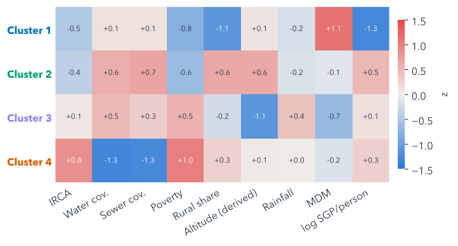
The highest-IRCA cluster, cluster 4, stands out on three things at once: piped-water coverage (−1.3 SD), poverty (+1.0 SD) and IRCA (+0.8 SD). Each cluster is such a combination, which is exactly what a single variable could not have found.
21.2 Name them by a rule
Names make clusters usable, and they also make them persuasive, so they need a rule that anyone can check. The analysis script’s name_rule() builds each name from three parts:
- Setting, tested in this order: “Rural” if fewer than 40% of the cluster’s rows are urban zones; otherwise “Cities and large towns” if its rural share is 0.5 SD or more below average, “Lowland towns” if its altitude is 0.5 SD or more below, “Highland towns” if 0.5 SD or more above, and plain “Towns” if none of these holds.
- Coverage: “low-coverage” if the cluster’s mean piped-water coverage is 0.5 SD or more below average.
- Risk: the Resolución 2115 band of the cluster’s median utility-supplied IRCA, the middle value when its zone-years are sorted by IRCA.
| Kind | Zone-years | Municipalities | Median IRCA (0–100) | |
|---|---|---|---|---|
| 1 | Cities and large towns, no-risk water | 2,271 | 284 | 1.6 |
| 2 | Highland towns, no-risk water | 3,750 | 558 | 4.0 |
| 3 | Lowland towns, low-risk water | 2,451 | 479 | 9.2 |
| 4 | Rural, low-coverage, high-risk water | 2,763 | 729 | 35.2 |
Because the rule reads the profile, the names never depend on which number k-means happened to give a cluster. Two words in them need care. “Low-coverage” is a relative position, not an absolute one: the rural cluster’s mean coverage is 30%, low but not zero, so “unserved” would overstate it. And the risk word describes the cluster’s median, not every zone-year in it: individual zone-years can sit in any band, and a median close to a band’s edge can flip the word.
Check every name against the heatmap and the profile table before you use it, and keep the rule beside the name in anything you publish. A name is a summary someone else will quote without the table. The thresholds, 40% and half a standard deviation, are choices too: a different one could change a name.
Tunja’s rural water scored in the high-risk band in its early years (Section 18.3). Before reading on, which cluster do you expect its rural zone to fall in, and what could put it somewhere else?
The rural cluster is the obvious guess. But k-means places a zone-year by all nine features at once, and several of them, such as the rural share and the altitude, belong to the municipality, so they are the same for both of Tunja’s zones. If those sit far from the rural cluster’s centre, they can outweigh the water.
21.3 Where Tunja lands
The cluster that holds all 16 of Tunja’s zone-years, urban and rural, now has a name: cluster 1 (cities and large towns), “Cities and large towns, no-risk water”. For the urban zone, it fits. For the rural zone, the label hides most of what Section 18.3 found. Its water scored in the high-risk band every year from 2010 to 2014, before the analysis’s window opens in 2016, and inside the window its utility-supplied IRCA is never in the no-risk band, and is in the medium band in three of the eight years.
Two things are at work. The risk word describes the cluster’s median, not each member, as Section 21.2 warned. And k-means puts each zone-year in the cluster whose centre is nearest over all nine features at once (Section 20.1), adding up the squared differences feature by feature. Table 21.2 splits that sum in two. On its own four features, IRCA, piped-water coverage, sewer coverage and poverty, Tunja’s rural zone sits nearer the centre of cluster 4 (rural), and two of those, the coverages, are fills (Section 19.2). The other five, rural share, altitude, rainfall, municipal performance and water transfers, are the municipality’s, the same for both zones. On those it sits far nearer cluster 1’s centre, by enough to outweigh the first four. The other two centres are farther still.
| Feature | Tunja, rural | Centre 1 | Centre 4 |
|---|---|---|---|
| IRCA | −0.2 | −0.5 | +0.8 |
| Piped-water coverage (filled) | −1.1 | +0.1 | −1.3 |
| Sewer coverage (filled) | −1.4 | +0.1 | −1.3 |
| Poverty | +0.3 | −0.8 | +1.0 |
| Squared distance, its own four | 5.0 | 1.7 | |
| Rural share | −2.1 | −1.1 | +0.3 |
| Altitude | +1.6 | +0.1 | +0.1 |
| Rainfall | −1.3 | −0.2 | +0.0 |
| Municipal performance | +1.5 | +1.1 | −0.2 |
| Water transfers | −2.3 | −1.3 | +0.3 |
| Squared distance, the shared five | 5.4 | 18.8 | |
| Squared distance, all nine | 10.5 | 20.5 |
It has company: 33% of that cluster’s zone-years are rural zones. A label describes a kind; to say anything about one member, go back to its rows.
21.4 Outcomes by cluster
Now the outcomes, which the clustering never used (Figure 21.2). Each line is a cluster’s median within each year, so a shift that moves every kind in one year cannot pass for a difference between kinds. Infant mortality is compared only in 2017–2019 and 2021–2023: its method changes in 2017, and 2020 looks like another source (the data’s README, caveat 8).
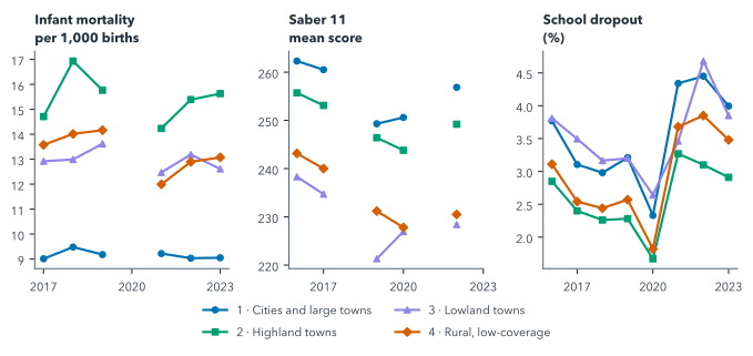
Gaps in the lines are years with no comparable value, drawn as gaps rather than joined across. Infant mortality and dropout are measured for a whole municipality but repeated on both zone rows, so they are counted once per municipality in each cluster and year: for these two the unit is the municipality-year, one municipality in one year, while the features and Saber 11 stay per zone-year.
Figure 21.3 puts the outcomes on the features’ scale: each outcome standardised within its year, a cell being the cluster’s mean z, with the mean itself in brackets.
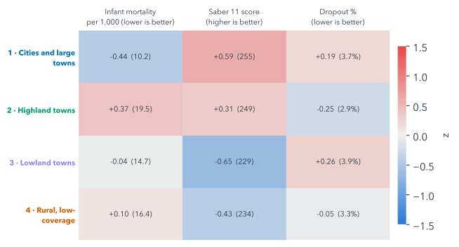
The paleness is the finding. No cluster’s mean outcome is more than 0.65 standard deviations from the average, against 1.32 for the features that formed them: the kinds differ less in outcomes than in what defines them. Part of this is by design: k-means chose the clusters to separate the features, so they should differ more on those than on anything else. Within that: the lowest recorded infant mortality is in cluster 1 (cities and large towns) and the highest in cluster 2 (highland towns); the best Saber 11 scores are in cluster 1 (cities and large towns); and the lowest dropout is in cluster 2 (highland towns).
Suppose unsafe water did harm infants’ health a great deal. Would you still expect the outcome heatmap to be paler than the features’?
Yes. k-means chose the clusters to separate the features, so they differ most on those by construction. The outcomes differ only as far as they go with the features, and small places’ noisy rates blur them further. Paleness alone is no evidence that water does not matter.
The highest recorded infant mortality is not in the cluster with the worst water, cluster 4 (rural). That is a good moment to slow down rather than to explain it away, because two things in the data push the same way. The first is small numbers. The rates of cluster 2 (highland towns) come from the smallest places of any kind, a median of 10,680 people per municipality-year, where a handful of deaths moves a rate a long way.
The second is what is missing. From 2017 the series looks like observed rates rather than modelled estimates, so a municipality where no infant died that year should show a rate of 0, yet no zero appears anywhere: a blank may be a recorded zero. 50% of this kind’s municipality-years are blank, against 32% of all clustered municipality-years. Leaving the blanks out drops what may be zeros, which raises small places’ averages most. That is selection on the outcome: whether a row is kept depends on the value being measured, so the rows kept are not typical. It may account for part of this kind’s place at the top. Small numbers, reporting and many other differences between the kinds all sit between a cluster’s water and its outcomes, and Chapter 22 takes that up directly.
21.5 Every variable, cluster by cluster
Means and medians hide overlap. Box plots show it: how each variable spreads within each cluster (Figure 21.4). Each box holds the middle half of a cluster’s values, with a solid line at the median and a dashed line at the mean, and its whiskers reach from the 5th to the 95th percentile, so they span the middle 90% of values. Features cover every zone-year 2016–2023; outcomes count in their years, municipal ones once per municipality.


The boxes make the overlap visible. Clusters differ sharply on the features that built them and overlap on the outcomes, and a gap between two clusters’ boxes is a description of the data, not an effect of water safety.
So the water analysis’s second question has an answer, and it is descriptive: infant mortality, exam scores and dropout do differ between the kinds of place, exam scores most, but by no more than 0.65 standard deviations in any cluster’s mean, and for every outcome the middle 90% of each kind’s values overlaps every other kind’s.
21.6 Building the interpretation
The normal route copies the finished outcome rules and names, as in Section 20.5:
Copy ../quarto-workshop/checkpoints/08-water-interpret/scripts/analysis.py over scripts/analysis.py (keep mine as scripts/analysis-before-08.py), run it with `uv run python scripts/analysis.py`, and show me the cluster names.copies · runs · writes outputs/outcomes_by_year.csv and outputs/cluster_profiles.csv
It should show four names, the ones in Table 21.1.
To build them instead (optional), two prompts: the outcome rules, then the profiles and names.
In scripts/analysis.py, add outcome rules: infant_mortality only in 2017–2019 and 2021–2023; infant_mortality and dropout_rate are municipal, so count each municipality once per `cluster` and `year`; saber11_mean stays per zone-year. Save outputs/outcomes_by_year.csv (median, n). Run it.Write outputs/cluster_profiles.csv: rows, municipalities, mean raw and z features, outcome medians and n under the same rules. Name each cluster by a rule: setting, relative coverage ("low-coverage" if mean z_water_coverage ≤ −0.5), median IRCA band. Show me the names.Whichever route you took, outputs/outcomes_by_year.csv should hold no infant-mortality rows for 2016 or 2020: the rules keep only the years whose method matches.
Both routes then add the interpretation to the clusters page:
Add to clusters.qmd a heatmap of the cluster mean z-scores (features × clusters, blue to red) and one line chart per outcome from outputs/outcomes_by_year.csv, with gaps, not joined lines, in missing years. Use the cluster names and colours. Render it.reload clusters.html in your browser
The page should show the heatmap, four clusters by nine features, and one chart per outcome, with the infant-mortality lines broken at 2020 and Saber 11’s at its unpublished years, such as 2018 and 2021.
While it renders: describe one cluster using two features that are not both coverage, then check whether its name says the same.
One good answer, from Figure 21.1: cluster 4, “Rural, low-coverage, high-risk water”, stands out on piped-water coverage (−1.3 SD) and poverty (+1.0 SD). Its name carries the coverage but not the poverty, one more reason to publish the profile beside the name.
21.7 Explorations in 3-D (optional)
The slide deck this book grew from has five more 3-D views of the outcomes the clustering never used, by cluster and year: dropout as terrain, clusters as hulls, the years stacked, clusters as orbits and dropout in Voronoi columns. They are exploratory pictures rather than evidence, and they run live in the published slides, starting with dropout as terrain.
Summary
- A cluster’s profile, its mean z-score on each feature, describes it as a combination of traits that no single variable could have found.
- A written rule names each cluster from its profile (setting, relative coverage, median IRCA band), so anyone can check the name.
- “Low-coverage” is relative and the risk word describes a median: Tunja’s rural zone, never no-risk inside the window, sits in a cluster named for no-risk water, carried there by what it shares with its urban zone.
- The outcomes, never used to form the clusters, differ between the kinds less than the features do, partly by design, and their distributions overlap.
- The highest recorded infant mortality is not where the water is worst, and small places and blank rates make that ranking fragile.
- All of it is description: a gap between kinds is not an effect of water safety.
Yet a description like this invites a causal reading. Chapter 22 tests the link inside each kind of place, where poverty, rurality and coverage are more alike than across the country.
Further reading
examples/water/scripts/analysis.py,name_rule(),profiles()andoutcomes_by_year(), in the repository.examples/water/data/README.md, caveat 8, on why infant mortality is compared only in 2017–2019 and 2021–2023.- matplotlib, boxplot: what the boxes, whiskers and means show (checked 2026-11-12).